Revision as of 21:02, 30 October 2025 (view source) Msanz (talk | contribs) ← Older edit		Revision as of 21:09, 30 October 2025 (view source) Msanz (talk | contribs) Newer edit →
Line 189:		Line 189:
	====3.1.3 Hydraulic conditions====		====3.1.3 Hydraulic conditions====
		+	The hydraulic conditions of the model are a constant discharge (left side of the model), as inlet, and a critical flow regime (right side of the model), as outlet. To implement so, we have to open the '''Boundary conditions manager''' ( ) and create a new by defining the ‘'''idval'''’ code (Fig. 4a). The ‘idval’ is a mandatory parameter, ‘name’ and ‘description’ are optional. IberGIS automatically will use this ‘idval’ as ‘Current scenario’. The manager window allows to store different inlet and outlet boundary conditions per scenario using the same ‘idval’ code.
		+	Before creating the boundary conditions, especially those that uses a timeseries like as inlet condition defined by a hydrograph, we must create previously through '''Non visual object manager''' window ( ). Go to ‘'''Timeseries'''’ tab and create the inlet condition by defining an increasing discharge from 0 to 0.1 m<sup>3</sup>/s in 60 s (Fig. 4b).
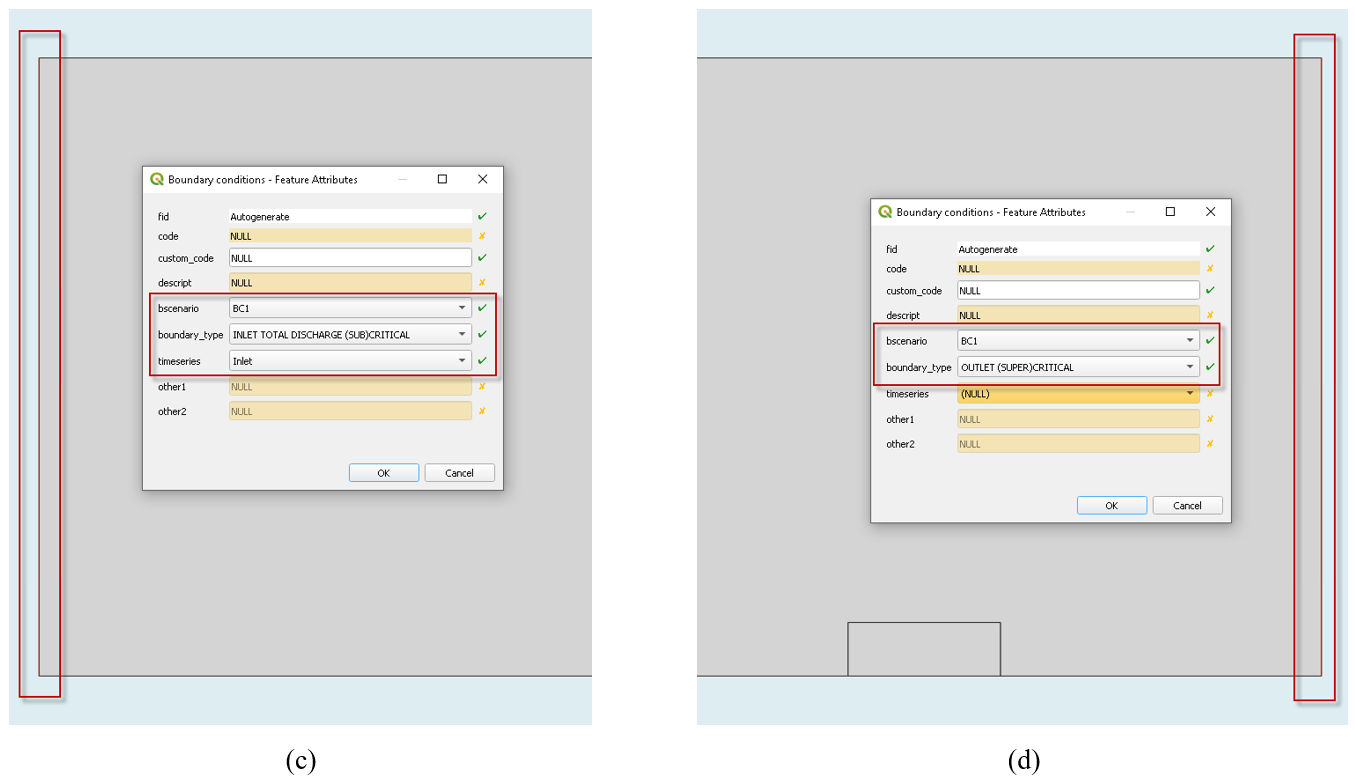
		+	The definition of the inlet/outlet condition can be carried out using the common options of QGIS by editing the layer called ‘'''Boundary conditions'''’. Select this layer and enable the editing mode ( ). Then, create a line ( ) that define the inlet boundary condition in the left side, as it is shown in Fig. 4c. In the Feature Attribute table of Boundary conditions select both the ‘bcscenario’ ('''BC1'''), ‘boundary_type’ ('''INLET TOTAL DISCHARGE (SUB)CRITICAL)''' and the ‘timeseries’ ('''Inlet'''). Repeat this process by selecting the opposite side for the outlet condition and defining the ‘bcscenario’ and the  ‘boundary_type’ as '''BC1''' and O'''UTLET (SUPER)CRITICAL''', respectively (Fig. 4d). Finish the edition mode and save it.
		+
		+	{| style="width: 95%;margin: 1em auto 0.1em auto;border-collapse: collapse;"
		+	|-
		+	|  style="text-align: center;width: 100%;"|[[File:Sanz-Ramos_et_al_2025a_9034_Fig_4a.png|1600px]]]
		+	|  style="text-align: center;width: 100%;"|[[File:Sanz-Ramos_et_al_2025a_5839_Fig_4b.png|1600px]]]
		+	|}
		+	<span style="text-align: center; font-size: 75%;">'''Fig. 3. Boundary conditions. (a) Creation of the current scenario. (b) Creation of the timeseries of the inlet conditions. (c) Implementation of the Inlet boundary condition. (d) Implementation of the Outlet boundary condition.'''</span>

---

Revision as of 21:09, 30 October 2025

Abstract

Urban drainage systems are facing increasing challenges due to climate change, urban growth, and the need for more sustainable water management. To address these issues, the Digital DRAIN project has developed an open-source tool that integrates different models within a GIS environment to analyse the performance of drainage systems. The tool helps assess both water flows and pollution, while also supporting the design of sustainable solutions and adaptation strategies. Delivered as the QGIS plugin IberGIS, it provides an accessible framework to improve urban water management and enhance resilience against floods and environmental impacts.

Keywords: urban drainage, 1D/2D modelling, Iber-SWMM, QGIS

Resumen

Los sistemas de drenaje urbano se enfrentan a retos cada vez mayores debido al cambio climático, el crecimiento urbano y la necesidad de una gestión del agua más sostenible. Para abordar estos problemas, el proyecto Digital DRAIN ha desarrollado una herramienta de código abierto que integra diversos modelos en un entorno SIG para analizar el rendimiento de los sistemas de drenaje. Esta herramienta permite evaluar tanto el caudal como la contaminación del agua, además de facilitar el diseño de soluciones sostenibles y estrategias de adaptación. Implementada como complemento de QGIS, IberGIS ofrece un marco accesible para mejorar la gestión del agua urbana y aumentar la resiliencia ante inundaciones e impactos ambientales.

Palabras clave: drenaje urbano, simulación 1D/2D, Iber-SWMM, QGIS

1 Introduction

In recent years, the planning, design, construction, and management of urban drainage elements has evolved towards an integrated approach, known as dual drainage. This process focuses on the joint understanding of all physical processes involved, both in terms of water quantity and quality, as well as surface and sewer network flows, and the final receiving environment (rivers, estuaries, seas, and oceans). This requires modelling and analysis tools that account for such coupling (dual drainage). Furthermore, these tools must address today’s global challenges, moving towards a more sustainable world, improving the ecological status of the environment, incorporating climate change adaptation strategies, and ensuring public safety in the face of natural phenomena such as floods.

Along these lines, the project entitled ‘Digital DRAIN. An Integrated Urban Drainage Model’ (DRAIN, CPP2021-008756) aims to develop an open-source, free modelling tool for analysing all processes of urban drainage, integrated within a graphical information system (GIS) environment. Its purpose is to assess hydraulic performance and the effects of diffuse pollution both on the surface, within the drainage network, and in the receiving environment. The tool will also include specific modules for the implementation of Sustainable Urban Drainage Systems (SuDS) and for analysing actions related to climate change adaptation.

The project derived in a plugin of QGIS, called IberGIS. This plugin is a full integration of the one-dimensional urban drainage software SWMM and a integration of the two-dimensional hydrodynamic software Iber, particularly its calculation module Iber-SWMM [1]. Thus, not all capabilities neither calculation modules of Iber are available. Only particular characteristics of the Iber-SWMM module are described below.

Data

Data to build-up the models presented in this document is stored here.

Important note

This document does not attempt to be a QGIS manual. Despite the whole model’s build-up process is properly defined, the input data might require a pre-process and previous knowledge in GIS environments. The authors encourage users to familiarise with QGIS by reading the documentation and, in case of general doubts, by contacting to the community.

2 Graphical user interface of IberGIS

2.1 Generalities

The graphical user interface (GUI) of the plugin IberGIS has been developed within the QGIS environment, and it follows the visual style guide. As for any plugin of QGIS, IberGIS can be installed through Plugins >> Manage and Install Plugins menu. Type “IberGIS” to search it and then click on Install Plugin button. Once installed, and according to the User’s Profile, it will be loaded automatically during the QGIS initialization.

2.2 Particularities

2.2.1 Model structure

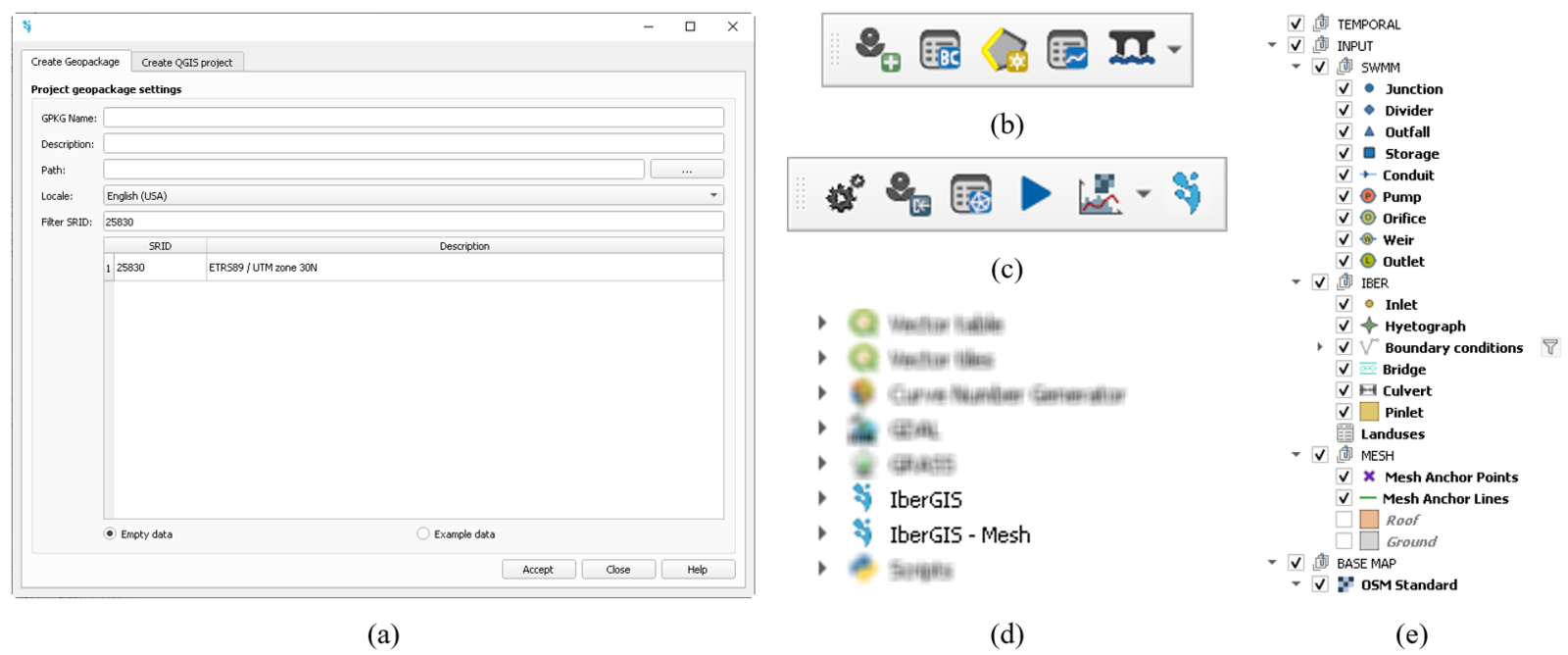
The IberGIS has a workflow fully integrated in the QGIS software. Once installed, the IberGIS button () will automatically appear in the toolbars of QGIS. Clicking there, a new window will ask for the geopackage and QGIS project creation (Fig. 1a).

After that, two new groups of toolbars of IberGIS will appear. One is related to the model’s build-up process (Fig. 1b) and the other to the model’s configuration, checks, run the simulation and visualize the results (Fig. 1c). A brief description of each option is detailed below:

• Import INP (). Imports the *.inp and *.ini files of any SWMM model.
• Boundary conditions manager (). Window that enables saving different boundary condition scenarios.
• Create boundary condition (). It automatizes the implementation of boundary conditions.
• Non visual objects manager (). Window that enables saving different non visual objects, such as timeseries, rules, etc.
• Bridges actions (). Options to implement and edit bridges.
• Options (). Main model options window.
• Generate INP (). Exports the current SWMM layers to a SWMM project.
• Mesh manager (). Window that enables saving different calculation mesh scenarios.
• Execute model (). Window that enables defining general options, selecting the calculation mesh and launch the simulation.
• Results (). Options to visualize the SWMM and Iber results.
• Check project (). Dialog that starts a check project.

Additionally, the Processing Toolbox will show two specific option for IberGIS plugin (Fig. 1d). Processing Toolbox >> IberGIS is related to automatize general procedures such as project checking, import necessary features (ground, roof, inlets layers), import results, and associate Iber inlets/roofs to SWMM junctions. The other one, accessible though 'Processing Toolbox >> IberGIS – Mesh, is a pack of particular options to obtain a well-conditioned calculation mesh.

]

Fig. 1. IberGIS workflow: (a) geopackage and project creation window; (b) build-up processing toolbar; (c) other options toolbar; (d) processing toolbox of IberGIS; (e) layers structure.

Note that any IberGIS model is saved in two files: a geopackage and the QGIS project. Both are linked and when the user opens the QGIS project, automatically it will look for the geopackage. Additionally, the geopackage contains the model itself, so the user can share it without the QGIS project.

2.2.2 Workflow

All this options and functionalities are oriented to facilitate the model build-up process. Since the model is saved in a unique geopackage, different kind of entities can be saved on it. On one hand, non-visual objects is managed in the abovementioned option (). On the other hand, the creation and edition of visual objects is based on a strict group of layers (Fig. 1e) that contains TEMPORAL information (e.g., meshes, results), INPUT data (e.g., data of SWMM and Iber models) and a BASE MAP image. It is mandatory to preserve the structure of the INPUT group, since other data saved in different layers will be omitted during the calculation process:

INPUT

• SWMM
  • Junction (layer of points)
  • Junction (layer of points)
  • Divider (layer of points)
  • Outfall (layer of points)
  • Storage (layer of points)
  • Conduit (layer of lines)
  • Pump (layer of lines)
  • Orifice (layer of lines)
  • Weir (layer of lines)
  • Outlet (layer of lines)
• IBER
  • Inlet (layer of points)
  • Hyetograph (layer of points)
  • Boundary conditions (layer of lines)
  • Bridge (layer of lines)
  • Culvert (layer of lines)
  • Pinlet (layer of surfaces)
  • Landuses (layer of dataset)
• MESH
  • Mesh anchor points (layer of points)
  • Mesh anchor lines (layer of lines)
  • Roof (layer of surfaces)
  • Ground (layer of surfaces)

The generation of this group of layers is automatic during the models creation. It can be edit manually, using the available tools of QGIS, or automatically, using the tools of IberGIS developed ad-hoc (Fig. 1d). Thus, a manual edition requires the generation of the geometric entities of some layer of INPUT group. I.e., if the user wants to simulate only a SWMM model, the proper layer must contain all the information together with the IBER and MESH data. Whereas, an Iber model, without sewer network, requires the definition of, at least, Ground and Boundary conditions layers. Roof layer is optional and when exists it can be linked directly to the Ground or to the Junction layer (if an Iber-SWMM model is simulated). In this sense, an Iber-SWMM model, i.e., a coupled urban drainage simulation, also requires the definition of the Inlet layer and, if there is no flow, the definition of the rainfall data, whether it is by hyetographs or rasters of rain.

It is worth noticing that raster data as topography or infiltration losses can be added to any layer’s group. During the Mesh generation process () these data, if exists in the project, can be selected. Other raster data, such as rainfall raster, must be defined as a timeseries () by defining the raster name per each time interval. The directory where the raster are located must be provided.

Previous to the simulation process (), a new folder will be created containing the files that calculation engine Iber-SWMM will be used to carry out the simulation, even save the results. As each simulation scenario can be saved independently, different folders will be created. Note if you share the model (*.gpkg and/or *.gps), the folder that contains the results will be lost. So, the model must be re-simulated to generate again the results or consider to share all this information together with the model.

2.2.3 Calculation engine

IberGIS uses the calculation engine of Iber and SWMM, and it particularly oriented to coupled simulations using the integrated module called Iber-SWMM [1]. The urban drainage models usually require high computational effort, especially in large urban areas, the computational time can be an enormous bottleneck. To solve this issue, the simulations are carried out using the parallelised version of Iber-SWMM for NVIDIA graphical power units (GPU) [2]. This allows accelerations in the computational time from 27 to 250 times faster than the single-threaded version.

Both models are freely distributed:

• SWMM: https://www.epa.gov/water-research/storm-water-management-model-swmm • Iber: https://www.iberaula.com/

2.3 Current and future versions

As above-mentioned, the current version of IberGIS is particularly oriented to address urban drainage and flood scenarios using, in a coupled way, two computational engines: Iber for the rainfall-runoff process and SWMM for the sewer network. Full capabilities and functionalities of the calculation engines are not currently available.

SWMM cannot be run independently since the rainfall-runoff process is carried out by Iber. Future versions might deal with these casuistic by generating a coupled and dual model, part of them being simulated with SWMM and the rest with Iber-SWMM.

Iber currently has 8 calculation modules [3] that works together with the hydrodynamic one, the principal module which the others depends on it. Only functionalities oriented to urban drainage of Iber-SWMM module are currently implemented in IberGIS. Despite that, some other functionalities, especially those related to the general hydrodynamics in flood scenarios assessment, are implemented such as bridges and culverts. Future versions might include other calculation modules of Iber.

3 Study cases

This User’s tutorial is composed by three examples: two real laboratory facility tests and a synthetic case. It is oriented to provide the elemental steps to build-up an IberGIS model, mainly to apply the Iber-SWMM calculation module for urban drainage applications.

3.1 Laboratory case: grate inlet testing platfrom

The experiment facility, located in the Hydraulic and Fluid Mechanics Laboratory of the Polytechnic University of Catalonia (UPC-BarcelonaTECH), consists in a 1:1-scale platform of 5.5 m-length and 3 m-width that represents the roadway of a street (Figure 1). This facility can be feed by a constant discharge up to 200 L/s and it can change its longitudinal and transverse slopes from 0 to 10 % and 0 to 4 %, respectively. It was originally designed to test the efficiency of longitudinal and transversal grate inlets [4–10]; nowadays, it is used to assess hazard criteria for objects that can be floated and transported during rainfall events in urban environments [11–14]. This exercise aims of familiarizing the user with the graphical interface and the structure of the layer, and to present other relevant information.

3.1.1 Data

The model will be build-up using the tools developed ad-hoc to facilitate the whole process. To that end, the following geometric entities are provided:

• Coordinates of the geometric entity (text

None additional geometric information is needed since the model will be created manually.

3.1.2 Model build-up

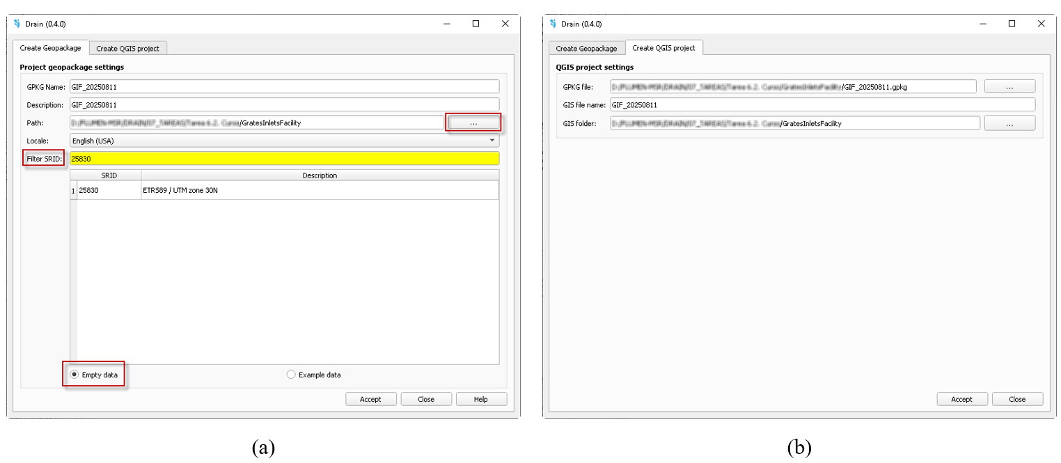
Once opened QGIS, load the IberGIS plugin by clicking on the icon , and the model generation window will appear (Fig. 2a). Please, enter the model name (GPKG Name) and a description. Then, define the location and the coordinate system using the Spatial Reference System Identifier (SRID), in this case 25830. After that, IberGIS asks for the QGIS project creation (Fig. 2b). This step is mandatory since it will automatically load the geopackage into the QGIS project

]

Fig. 2. Model generation window: (a) creation of the geopackage tab; (b) creation of the QGIS project tab.

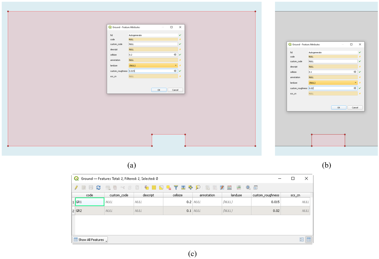
The geometry of the facility is defined by 8 points that we have to load as Delimited Text Layer bye the menu Layer >> Add Layer >> Delimited Text Layer. Now, we have to select start editing () the layer called ‘Ground’ located in the group INPUT > IBER, which contains the main information of model geometry. Add Polygon Feature () by selecting the imported points and creating a polygon that represents the street part of the laboratory facility platform (Fig. 3). After finishing the geometry, the Feature Attribute table of ‘Ground’ layer will appear asking for the geometry properties. We can introduce a ‘cellsize’ of 0.2 m and a ‘custom_roughness’ of 0.015 s·m^-1/3 (Fig. 3a). Repeat this action to create the polygon that represents de grate inlet geometry and introducing a ‘cellsize’ and ‘custom_roughness’ of 0.1 m and 0.02, respectively (Fig. 3b). Finish editing mode to save the changes into ‘Ground’ layer. Note, ‘Enable Snapping’ () option will facilitate the creation of the model.

]

Fig. 3. ‘Ground’ layer creation: (a) generation of the platform geometry; (b) generation of the grate inlet geometry; (c) View of the attribute table of ‘Ground’ layer.

This geometry corresponds to the grate inlet called ‘Barcelona1’, commonly used in Barcelona city and already experimentally and numerically tested in this facility (e.g., [9,10,15–17]). Open the attribute table of ‘Ground’ layer to verify that, indeed, the geometry is properly saved together with the properties that we defined previously (Fig. 3c). Now, we can edit both the geometry and the properties of each geometrical feature of this layer.

We can hide or delete the auxiliary layer of points used to create the polygons of ‘Ground’ layer.

3.1.3 Hydraulic conditions

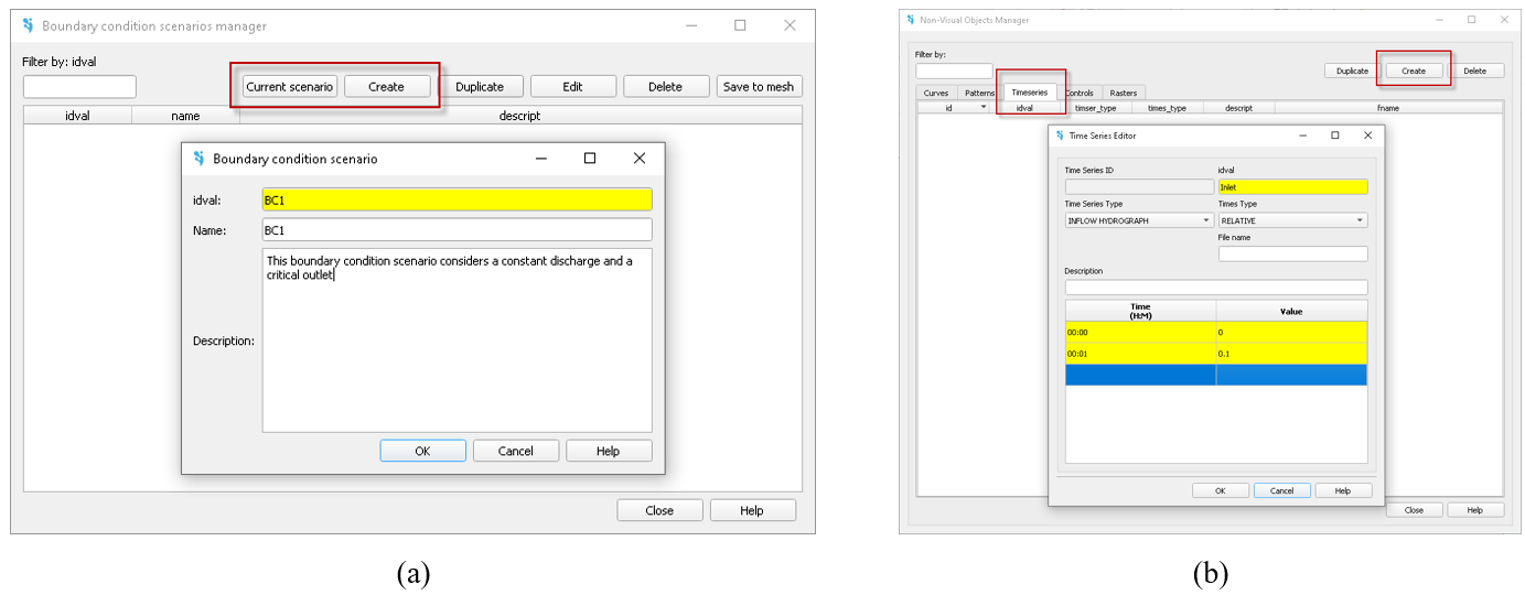
The hydraulic conditions of the model are a constant discharge (left side of the model), as inlet, and a critical flow regime (right side of the model), as outlet. To implement so, we have to open the Boundary conditions manager ( ) and create a new by defining the ‘idval’ code (Fig. 4a). The ‘idval’ is a mandatory parameter, ‘name’ and ‘description’ are optional. IberGIS automatically will use this ‘idval’ as ‘Current scenario’. The manager window allows to store different inlet and outlet boundary conditions per scenario using the same ‘idval’ code.

Before creating the boundary conditions, especially those that uses a timeseries like as inlet condition defined by a hydrograph, we must create previously through Non visual object manager window ( ). Go to ‘Timeseries’ tab and create the inlet condition by defining an increasing discharge from 0 to 0.1 m³/s in 60 s (Fig. 4b).

The definition of the inlet/outlet condition can be carried out using the common options of QGIS by editing the layer called ‘Boundary conditions’. Select this layer and enable the editing mode ( ). Then, create a line ( ) that define the inlet boundary condition in the left side, as it is shown in Fig. 4c. In the Feature Attribute table of Boundary conditions select both the ‘bcscenario’ (BC1), ‘boundary_type’ (INLET TOTAL DISCHARGE (SUB)CRITICAL) and the ‘timeseries’ (Inlet). Repeat this process by selecting the opposite side for the outlet condition and defining the ‘bcscenario’ and the ‘boundary_type’ as BC1 and OUTLET (SUPER)CRITICAL, respectively (Fig. 4d). Finish the edition mode and save it.

]

]

Fig. 3. Boundary conditions. (a) Creation of the current scenario. (b) Creation of the timeseries of the inlet conditions. (c) Implementation of the Inlet boundary condition. (d) Implementation of the Outlet boundary condition.

References

[1] E. Bladé, L. Cea, G. Corestein, E. Escolano, J. Puertas, E. Vázquez-Cendón, J. Dolz, A. Coll, Iber: herramienta de simulación numérica del flujo en ríos, Rev. Int. Métodos Numéricos Para Cálculo y Diseño En Ing. 30 (2014) 1–10. https://doi.org/10.1016/j.rimni.2012.07.004.

[2] M. Sanz-Ramos, E. Bladé, P. Oller, G. Furdada, Numerical modelling of dense snow avalanches with a well-balanced scheme based on the 2D shallow water equations, J. Glaciol. (2023) 1–17. https://doi.org/10.1017/jog.2023.48.

[3] M. Sanz-Ramos, E. Bladé, M. Sánchez-Juny, El rol de los términos de fricción y cohesión en la modelización bidimensional de fluidos no Newtonianos: avalanchas de nieve densa, Ing. Del Agua. 27 (2023) 295–310. https://doi.org/10.4995/ia.2023.20080.

[4] M. Sanz-Ramos, C.A. Andrade, P. Oller, G. Furdada, E. Bladé, E. Martínez-Gomariz, Reconstructing the Snow Avalanche of Coll de Pal 2018 (SE Pyrenees), GeoHazards. 2 (2021) 196–211. https://doi.org/10.3390/geohazards2030011.

[5] V. Ruiz-Villanueva, B. Mazzorana, E. Bladé, L. Bürkli, P. Iribarren-Anacona, L. Mao, F. Nakamura, D. Ravazzolo, D. Rickenmann, M. Sanz-Ramos, M. Stoffel, E. Wohl, Characterization of wood-laden flows in rivers, Earth Surf. Process. Landforms. 44 (2019) 1694–1709. https://doi.org/10.1002/esp.4603.

[6] M. Sanz-Ramos, J.J. Vales-Bravo, E. Bladé, M. Sánchez-Juny, Reconstructing the spill propagation of the Aznalcóllar mine disaster, Mine Water Environ. 43 (2024). https://doi.org/10.1007/s10230-024-01000-5.

[7] M. Sanz-Ramos, E. Bladé, M. Sánchez-Juny, T. Dysarz, Extension of Iber for Simulating Non–Newtonian Shallow Flows: Mine-Tailings Spill Propagation Modelling, Water. 16 (2024) 2039. https://doi.org/10.3390/w16142039.

[8] M. Sanz-Ramos, L. Cea, E. Bladé, D. López-Gómez, E. Sañudo, G. Corestein, G. García-Alén, J. Aragón-Hernández, Iber v3. Reference manual and user’s interface of the new implementations, CIMNE, 2022. https://doi.org/10.23967/iber.2022.01.

[9] Y. Ni, Z. Cao, Q. Liu, Mathematical modeling of shallow-water flows on steep slopes, J. Hydrol. Hydromechanics. 67 (2019) 252–259. https://doi.org/10.2478/johh-2019-0012.

[10] A. Maranzoni, M. Tomirotti, New formulation of the two-dimensional steep-slope shallow water equations. Part I: Theory and analysis, Adv. Water Resour. 166 (2022) 104255. https://doi.org/10.1016/j.advwatres.2022.104255.

[11] D. Zugliani, G. Rosatti, TRENT2D❄: An accurate numerical approach to the simulation of two-dimensional dense snow avalanches in global coordinate systems, Cold Reg. Sci. Technol. 190 (2021) 103343. https://doi.org/10.1016/j.coldregions.2021.103343.

[12] V. Te Chow, Open-Channel Hydraulics, McGraw-Hill Book Company Inc. New York, USA, 1959.

[13] S.B. Savage, K. Hutter, The motion of a finite mass of granular material down a rough incline, J. Fluid Mech. 199 (1989) 177–215. https://doi.org/10.1017/S0022112089000340.

[14] M. Christen, J. Kowalski, P. Bartelt, RAMMS: Numerical simulation of dense snow avalanches in three-dimensional terrain, Cold Reg. Sci. Technol. 63 (2010) 1–14. https://doi.org/10.1016/j.coldregions.2010.04.005.

[15] M.E. Eglit, K.S. Demidov, Mathematical modeling of snow entrainment in avalanche motion, Cold Reg. Sci. Technol. 43 (2005) 10–23. https://doi.org/10.1016/j.coldregions.2005.03.005.

[16] J. Castelló, Enhancement and application of numerical methods for snow avalanche modelling, Master thesis. Universitat Politècnica de Catalunya. Barcelona, Spain, 2020.

[17] K. Msheik, Non-Newtonian Fluids: Modeling and Well-Posedness, Universite Grenoble Alpes, Saint-Martin-d’Hères, France, 2020. https://hal.archives-ouvertes.fr/tel-03099969.

[18] P.Y. Julien, C.A. León, Mudfloods, mudflows and debrisflows, classification in rheology and structural design, in: Int. Work. Debris Flow Disaster 27 November–1 December 1999, 2000: pp. 1–15.

[19] T. Takahashi, Debris flow: mechanics and hazard mitigation, in: ROC-JAPAN Jt. Semin. Mul- Tiple Hazards Mitig., National Taiwan Univerisity, Taipei, Taiwan, ROC, 1985: pp. 1075–1092.

[20] A. Laenen, R.P. Hansen, Simulation of three lahars in the Mount St. Helens area, Washington, using a one-dimensional, unsteady-state streamflow model, 1988. https://doi.org/https://doi.org/10.3133/wri884004.

[21] M. Syarifuddin, S. Oishi, R.I. Hapsari, D. Legono, Empirical model for remote monitoring of rain-triggered lahar at Mount Merapi, J. Japan Soc. Civ. Eng. Ser. B1 (Hydraulic Eng. 74 (2018) I_1483-I_1488. https://doi.org/10.2208/jscejhe.74.I_1483.

[22] A.R. Darnell, J.C. Phillips, J. Barclay, R.A. Herd, A.A. Lovett, P.D. Cole, Developing a simplified geographical information system approach to dilute lahar modelling for rapid hazard assessment, Bull. Volcanol. 75 (2013) 713. https://doi.org/10.1007/s00445-013-0713-6.

[23] E.C. Bingham, An investigation of the laws of plastic flow, Bull. Bur. Stand. 13 (1916) 309–353. https://doi.org/10.6028/bulletin.304.

[24] M. Pastor, B. Haddad, G. Sorbino, S. Cuomo, V. Drempetic, A depth‐integrated, coupled SPH model for flow‐like landslides and related phenomena, Int. J. Numer. Anal. Methods Geomech. 33 (2009) 143–172. https://doi.org/10.1002/nag.705.

[25] H. Chen, C.F. Lee, Runout Analysis of Slurry Flows with Bingham Model, J. Geotech. Geoenvironmental Eng. 128 (2002) 1032–1042. https://doi.org/10.1061/(ASCE)1090-0241(2002)128:12(1032).

[26] D. Naef, D. Rickenmann, P. Rutschmann, B.W. McArdell, Comparison of flow resistance relations for debris flows using a one-dimensional finite element simulation model, Nat. Hazards Earth Syst. Sci. 6 (2006) 155–165. https://doi.org/10.5194/nhess-6-155-2006.

[27] A. Voellmy, Über die Zerstörungskraft von Lawinen, Schweizerische Bauzeitung. 73 (1955) 15. https://doi.org/10.5169/seals-61891.

[28] P. Bartelt, C.V. Valero, T. Feistl, M. Christen, Y. Bühler, O. Buser, Modelling cohesion in snow avalanche flow, J. Glaciol. 61 (2015) 837–850. https://doi.org/10.3189/2015JoG14J126.

[29] G. Macedonio, M.T.T. Pareschi, Numerical simulation of some lahars from Mount St. Helens, J. Volcanol. Geotherm. Res. 54 (1992) 65–80. https://doi.org/10.1016/0377-0273(92)90115-T.

[30] J.S. O’Brien, P.Y. Julien, Laboratory Analysis of Mudflow Properties, J. Hydraul. Eng. 114 (1988) 877–887. https://doi.org/10.1061/(ASCE)0733-9429(1988)114:8(877).

[31] W.H. Herschel, R. Bulkley, Konsistenzmessungen von Gummi-Benzollösungen, Kolloid-Zeitschrift. 39 (1926) 291–300. https://doi.org/10.1007/bf01432034.

[32] L. Dreier, Y. Bühler, W. Steinkogler, T. Feistl, M. Christen, P. Bartelt, Modelling Small and Frequent Avalanches, in: Int. Snow Sci. Work. 2014 Proc., 29 Sep - 3 Oct, Banff, Canada, 2014: p. 8. http://arc.lib.montana.edu/snow-science/item/2128.

[33] V. Medina, M. Hürlimann, A. Bateman, Application of FLATModel, a 2D finite volume code, to debris flows in the northeastern part of the Iberian Peninsula, Landslides. 5 (2008) 127–142. https://doi.org/10.1007/s10346-007-0102-3.

[34] M. Eglit, A. Yakubenko, J. Zayko, A Review of Russian Snow Avalanche Models—From Analytical Solutions to Novel 3D Models, Geosciences. 10 (2020) 77. https://doi.org/10.3390/geosciences10020077.

[35] M. Garcia, G. Parker, Entrainment of Bed Sediment into Suspension, J. Hydraul. Eng. 117 (1991) 414–435. https://doi.org/10.1061/(ASCE)0733-9429(1991)117:4(414).

[36] P. Bartelt, B. Salm, U. Gruber, Calculating dense-snow avalanche runout using a Voellmy-fluid model with active/passive longitudinal straining, J. Glaciol. 45 (1999) 242–254. https://doi.org/10.3189/s002214300000174x.

[37] C.J. Keylock, M. Barbolini, Snow avalanche impact pressure - vulnerability relations for use in risk assessment, Can. Geotech. J. 38 (2011) 227–238. https://doi.org/10.1139/t00-100.

[38] F. Rudolf-Miklau, S. Sauermoser, A.I. Mears, F. Rudolf‐Miklau, S. Sauermoser, A.I. Mears, The Technical Avalanche Protection Handbook, Wiley, Berlin, Germany, 2014. https://doi.org/10.1002/9783433603840.

Document