| Line 36: | Line 36: | ||
Along these lines, the project entitled ‘Digital DRAIN. An Integrated Urban Drainage Model’ (DRAIN, CPP2021-008756) aims to develop an open-source, free modelling tool for analysing all processes of urban drainage, integrated within a graphical information system (GIS) environment. Its purpose is to assess hydraulic performance and the effects of diffuse pollution both on the surface, within the drainage network, and in the receiving environment. The tool will also include specific modules for the implementation of Sustainable Urban Drainage Systems (SuDS) and for analysing actions related to climate change adaptation. | Along these lines, the project entitled ‘Digital DRAIN. An Integrated Urban Drainage Model’ (DRAIN, CPP2021-008756) aims to develop an open-source, free modelling tool for analysing all processes of urban drainage, integrated within a graphical information system (GIS) environment. Its purpose is to assess hydraulic performance and the effects of diffuse pollution both on the surface, within the drainage network, and in the receiving environment. The tool will also include specific modules for the implementation of Sustainable Urban Drainage Systems (SuDS) and for analysing actions related to climate change adaptation. | ||
| − | The project derived in a plugin of [https://qgis.org/ QGIS], called IberGIS. This plugin is a full integration of the one-dimensional urban drainage software [https://www.epa.gov/water-research/storm-water-management-model-swmm SWMM] and a integration of the two-dimensional hydrodynamic software [http://www.iberaula.com Iber | + | The project derived in a plugin of [https://qgis.org/ QGIS], called IberGIS. This plugin is a full integration of the one-dimensional urban drainage software [https://www.epa.gov/water-research/storm-water-management-model-swmm SWMM] and a integration of the two-dimensional hydrodynamic software [http://www.iberaula.com Iber], particularly its calculation module Iber-SWMM [<span id='cite-_Bib001'></span>[[#_Bib001|1]]]. Thus, not all capabilities neither calculation modules of Iber are available. Only particular characteristics of the Iber-SWMM module are described below. |
'''Data''' | '''Data''' | ||
| Line 64: | Line 64: | ||
[[File:Sanz-Ramos_et_al_2025a_7022_Icon_Iber.png]] | [[File:Sanz-Ramos_et_al_2025a_7022_Icon_Iber.png]] | ||
) will automatically appear in the toolbars of QGIS. Clicking there, a new window will ask for the geopackage and QGIS project creation (Fig. 1a). | ) will automatically appear in the toolbars of QGIS. Clicking there, a new window will ask for the geopackage and QGIS project creation (Fig. 1a). | ||
| + | |||
| + | After that, two new groups of toolbars of IberGIS will appear. One is related to the model’s build-up process (Fig. 1b) and the other to the model’s configuration, checks, run the simulation and visualize the results (Fig. 1c). A brief description of each option is detailed below: | ||
| + | |||
| + | * Bulleted list item hola | ||
| + | * Bulleted list item caracola | ||
{| style="width: 84%;margin: 1em auto 0.1em auto;border-collapse: collapse;" | {| style="width: 84%;margin: 1em auto 0.1em auto;border-collapse: collapse;" | ||
Revision as of 15:18, 30 October 2025
Abstract
Urban drainage systems are facing increasing challenges due to climate change, urban growth, and the need for more sustainable water management. To address these issues, the Digital DRAIN project has developed an open-source tool that integrates different models within a GIS environment to analyse the performance of drainage systems. The tool helps assess both water flows and pollution, while also supporting the design of sustainable solutions and adaptation strategies. Delivered as the QGIS plugin IberGIS, it provides an accessible framework to improve urban water management and enhance resilience against floods and environmental impacts.
Keywords: urban drainage, 1D/2D modelling, Iber-SWMM, QGIS
Resumen
Los sistemas de drenaje urbano se enfrentan a retos cada vez mayores debido al cambio climático, el crecimiento urbano y la necesidad de una gestión del agua más sostenible. Para abordar estos problemas, el proyecto Digital DRAIN ha desarrollado una herramienta de código abierto que integra diversos modelos en un entorno SIG para analizar el rendimiento de los sistemas de drenaje. Esta herramienta permite evaluar tanto el caudal como la contaminación del agua, además de facilitar el diseño de soluciones sostenibles y estrategias de adaptación. Implementada como complemento de QGIS, IberGIS ofrece un marco accesible para mejorar la gestión del agua urbana y aumentar la resiliencia ante inundaciones e impactos ambientales.
Palabras clave: drenaje urbano, simulación 1D/2D, Iber-SWMM, QGIS
1 Introduction
In recent years, the planning, design, construction, and management of urban drainage elements has evolved towards an integrated approach, known as dual drainage. This process focuses on the joint understanding of all physical processes involved, both in terms of water quantity and quality, as well as surface and sewer network flows, and the final receiving environment (rivers, estuaries, seas, and oceans). This requires modelling and analysis tools that account for such coupling (dual drainage). Furthermore, these tools must address today’s global challenges, moving towards a more sustainable world, improving the ecological status of the environment, incorporating climate change adaptation strategies, and ensuring public safety in the face of natural phenomena such as floods.
Along these lines, the project entitled ‘Digital DRAIN. An Integrated Urban Drainage Model’ (DRAIN, CPP2021-008756) aims to develop an open-source, free modelling tool for analysing all processes of urban drainage, integrated within a graphical information system (GIS) environment. Its purpose is to assess hydraulic performance and the effects of diffuse pollution both on the surface, within the drainage network, and in the receiving environment. The tool will also include specific modules for the implementation of Sustainable Urban Drainage Systems (SuDS) and for analysing actions related to climate change adaptation.
The project derived in a plugin of QGIS, called IberGIS. This plugin is a full integration of the one-dimensional urban drainage software SWMM and a integration of the two-dimensional hydrodynamic software Iber, particularly its calculation module Iber-SWMM [1]. Thus, not all capabilities neither calculation modules of Iber are available. Only particular characteristics of the Iber-SWMM module are described below.
Data
Data to build-up the models presented in this document is stored here.
Important note
This document does not attempt to be a QGIS manual. Despite the whole model’s build-up process is properly defined, the input data might require a pre-process and previous knowledge in GIS environments. The authors encourage users to familiarise with QGIS by reading the documentation and, in case of general doubts, by contacting to the community.
2 Graphical user interface of IberGIS
2.1 Generalities
The graphical user interface (GUI) of the plugin IberGIS has been developed within the QGIS environment, and it follows the visual style guide. As for any plugin of QGIS, IberGIS can be installed through Plugins >> Manage and Install Plugins menu. Type “IberGIS” to search it and then click on Install Plugin button. Once installed, and according to the User’s Profile, it will be loaded automatically during the QGIS initialization.
2.2 Particularities
2.3.1 Velocity-dependent terms
The IberGIS has a workflow fully integrated in the QGIS software. Once installed, the IberGIS button (
![]() ) will automatically appear in the toolbars of QGIS. Clicking there, a new window will ask for the geopackage and QGIS project creation (Fig. 1a).
) will automatically appear in the toolbars of QGIS. Clicking there, a new window will ask for the geopackage and QGIS project creation (Fig. 1a).
After that, two new groups of toolbars of IberGIS will appear. One is related to the model’s build-up process (Fig. 1b) and the other to the model’s configuration, checks, run the simulation and visualize the results (Fig. 1c). A brief description of each option is detailed below:
- Bulleted list item hola
- Bulleted list item caracola
|
|
| (a) | (b) |
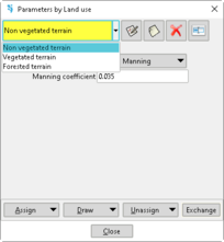
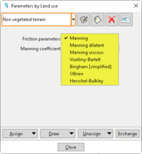
Fig. 1. Land uses windows: (a) database of land uses for non-Newtonian flows; (b) list of velocity-dependent parameters according to each rheological model.
2.3 Implementation of rheological properties of the fluid
As mentioned previously, there is a different way to implement the rheological properties of the fluid in Iber-NNF.
2.3.1 Velocity-dependent terms
Velocity-dependent terms of the rheological model must be implemented as a friction slope at each mesh element (Data >> Roughness >> Friction slope…). These parameters can be defined manually or automatically (by a raster file), and are associated to the concept known as ‘Land use’; thus, they can vary spatially.

|

|
| (a) | (b) |
Fig. 1. Land uses windows: (a) database of land uses for non-Newtonian flows; (b) list of velocity-dependent parameters according to each rheological model.
2.3.2 Non–Velocity-dependent terms
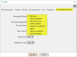
By contrast, non–Velocity-dependent terms can be interpreted as a characteristic of the fluid; thus, they cannot vary spatially –perhaps temporally– and they must be defined as a constant value (Data >> Problem data > Non Newtonian Fluid). This is the case of the flow density, the pressure factor, the Coulomb friction coefficient, the yield stress, etc.
Fig. 2. Problem data window. Non-Newtonian fluid tab allows the selection of the rheological model to be used and other properties.
2.4 Stop criterion
The detention of any fluid is consequence of a balance between resistance and driving forces. Iber-NNF uses an ad hoc numerical scheme that allows the stop of the fluid according to the fluid properties [2], i.e. the rheological model.
Another popular numerical model uses a stopping criterion based on controlling the momentum, where the fluid is made to stop when its momentum is lower than a user-defined fraction of its maximum momentum. However, this criterion lacks a physical basis, as the maximum momentum depends on the avalanche’s characteristics at very different location and time than those when it stops.
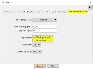
Both stop criterion are implemented into Iber-NNF; nevertheless, we encourage to use the ‘Rheology based’ criterion because is physically based.
Fig. 3. Problem data window. Selection of the stop criterion.
3 Governing equations
This section is a brief description of the governing equations of Iber-NNF. Further details about this hydrodynamic module and the numerical scheme used to solve the equations can be found in Sanz-Ramos et al. [2].
3.1 2D shallow water equations for non-Newtonian shallow flows
Iber-NNF solves a particular case of the two-dimensional shallow water equations (2D-SWE), a hyperbolic nonlinear system of three partial differential equations described in Equation (1):
|
|
(1) |
where is the water depth, and are the two components of the specific discharge, is the gravitational acceleration, and are the two bottom slope components computed as , where is the bed elevation, and and are the two friction slope components computed throughout the rheological model. The friction forces exerted over an inclined bed and the pressure terms can be corrected by replacing the gravity acceleration by [9,10,11]. Since the hydrostatic and isotropic pressure distribution cannot be assumed for non-Newtonian flows, as it is done for free surface water flows [12], a factor multiplying the pressure terms in the momentum equations was applied [13]. A value equal to 1 implies hydrostatic and isotropic pressure distribution. The term is entrainment, a process by which solid particles or fragments become incorporated into a moving fluid. The current code partially integrates entrainment formulas based on flow velocity criterion [14], flow height criterion [15] and bed shear stress criterion [16]. The acknowledgment of entrainment is essential for ensuring reliable outcomes and, thus, preventing the underestimation of the volume of snow descending a slope.
3.2 Rheological models
Rheological models to describe both dynamic and static phase of non–Newtonian shallow flows exist for a wide field of applications. In particular, for those related to environmental flows, and more specially for shallow flows, several rheological models have been developed to describe the relationship between the shear stress and the shear rate [17].
From the simplest Potential law to the full –and complex– Bingham model, several rheological models exist in the literature, the development of each one being oriented to achieve a particular reproduction of a fluid behaviour. The aim of Iber-NNF is not to include as rheological models as possible –or exist–; however, there are some models that, although they have been omitted, can be easily integrated into the proposed numerical scheme by slightly adapting the code. This would allow a broader simulation of the behaviour of non–Newtonian shallow fluids.
Two hypotheses are usually considered in non-Newtonian shallow flows modelling: a monophasic fluid, in which the fluid is formed by a unique phase where all components are perfectly mixed, and shear stress grouping, in which the effect of different shear stresses are grouped as five components of a single term [18] as follows:
|
|
(2) |
where represents the dispersive term, the turbulent term, the viscous term, the Mohr–Coulomb terms, and the cohesive term. In these components, the appropriate rheological model for the particular purpose of each work is obtained by selecting one or several components of Equation (2).
Iber-NNF integrates several rheological models to represent the resistance forces that act against flow motion of non–Newtonian flows, such as mudflows, debris flows, snow avalanches, lahars, etc. [2,3,4,5,6,7]. The following sections describe the rheological models implemented expressed in friction slope form ( ).
3.2.1 Manning
The Manning rheological model, an empirical equation widely utilised in hydraulics and hydrology, applies to uniform flow in open channels and is a function of the channel velocity, flow area and channel slope:
|
|
(3) |
where is the Manning coefficient, is the flow velocity and is the flow depth. It is related to turbulent friction ( ), being utilised by several authors for simulating hyperconcentrated flows [19,20,21,22]. The unique value for calibration is the Manning coefficient ( ).
3.2.2 Bingham (simplified)
Since the proposal of the Bingham rheological model [23], several approaches have been introduced to deal with the difficulties on directly obtaining the shear stress proportional to the flow velocity [24]. Assuming an incompressible and homogeneous flow [25,26], the following expression for the viscous ( ) and the Mohr–Coulomb ( ) contributions:
|
|
(4) |
where is the yield stress, is the fluid density, is the flow depth, is the fluid viscosity, is the flow velocity, and is the gravitational acceleration.
3.2.3 Voellmy
Voellmy [27] presented a rheological model that considers the turbulent ( ) and the Mohr–Coulomb ( ) terms as follows:
|
|
(5) |
where is the turbulent friction coefficient, is the Coulomb friction coefficient, is the flow depth and is the flow velocity.
3.2.4 Bartelt
Bartelt et al. [28] developed a new resistance term related to the cohesion, a physical property of the fluid. This rheological model is commonly used together with the Voellmy model, and expresses as follows:
|
|
(6) |
where is the fluid density, is the gravitational acceleration, is the flow depth, is the cohesion, and is the Coulomb friction coefficient.
3.2.5 Dilatant
Similarly to the Manning rheological models, and considering constant sediment concentration and uniform flow, Macedonio and Pareschi [29] derived the following expression: , where is the yield stress, is a proportionality coefficient and is the flow behaviour index.
When = 2 a dilatant flow behaviour is expected:
|
|
(7) |
3.2.6 Viscous
Macedonio and Pareschi [29] also presented the application of the Manning equation to viscous flows by particularizing the parameter = 1. This allows for the representation of viscous flows:
|
|
(8) |
3.2.7 O’Brien
On the other hand, O’Brien and Julien [30] derived an expression for the representation of the shear stress of mudflows, being a quadratic equation that integrates the Mohr–Coulomb term ( ), the viscous term ( ) and the turbulent term ( ) as follows:
|
|
(9) |
where is the yield stress, is the fluid density, is the gravitational acceleration, is the flow depth, is a resistance parameter, is the flow viscosity, is the flow velocity, and is the Manning coefficient.
3.2.8 Herschel-Bulkley
The formulation of Herschel and Bulkley [31] is a generalization of various expressions in which, depending on the value of the coefficient , dilatant, viscous, plastic, etc. behaviours can be derived. This formula follows the following expression:
|
|
(10) |
where is the yield stress, is the fluid density, is the gravitational acceleration, is the flow depth, is a consistency parameter, and is the flow velocity.
3.3 Entrainment
The entrainment is a relevant phenomenon in non-Newtonian flow dynamic modelling because the shear stress between the moving fluid and the terrain generally erode the bottom. This eroded material is then aggregated to the bulk, and might affect it properties (e.g., fluid density) and behaviour.
The effects of entrainment extend beyond altering mass and energy balances. Predicted velocities along the bulk path and the kinetic energy upon reaching the runout zone are also affected. These changes directly influence runout distances and have substantial implications for hazard and risk mapping. Particularly for snow avalanche modelling, entrainment leads to higher predicted flow heights and volumes of avalanches [15,32,33,34,35].
Accurate predictions are crucial for designing infrastructure, such as barriers or dams, as incorrect estimations may result in inadequate protection or increased costs. Therefore, precise consideration of entrainment is essential for determining runout distances and optimizing infrastructure design to mitigate hazards effectively.
3.3.1 Velocity model
This is a simple model that considers mass entrainment as function of the flow velocity. In contrast with another popular model, Iber-NNF considers entrainment when the flow velocity is greater than a threshold ( ).
|
|
(11) |
where is the entrainment rate, which commonly range from 5 to 40·10-5.
3.3.2 Height model
In this model, the entrainment depends on the load of the underlying snow cover as long as its height reaches a fixed minimum value ( ); otherwise, the entrainment will be considered inexistent [15]. This model also integrates an upper limit for the height based on the dry friction law to avoid the dry friction increasing limitless [36]:
|
|
(12) |
where is the entrainment rate, which commonly range from 1 to 8·10-3 s-1, and being the maximum avalanche flux height at which yielding at the basal surface occurs:
|
|
(13) |
3.3.3 Squared velocity model
This equation is similar to the velocity model although the entrainment rate is considered to vary with the squared velocity of the avalanche [15]:
|
|
(14) |
where is the entrainment rate, which commonly range from 4 to 32·10-6.
3.3.4 Bed shear stress model
Similar to how the sediment transport is computed, a new equation to calculate the entrainment as a function of the bed shear stress between the lower snow layer and the avalanche:
|
|
(15) |
where is the entrainment rate, which a range from 1.5 to 12·10-6 m·s-1·Pa-1 is proposed [16].
4 Results
As in the hydrodynamic module for water flows, Iber-NNF also integrates flow depths, velocities, elevation, etc. However, particular results can be activated through Data >> Problem data >> NonNewtonian fluid tab, such as extra topographical information (terrain slope) and impact forces [37,38]. This results essentially applies for dense snow avalanche modelling, but they are not limited to.
Particularly for impact forces, Iber-NNF calculates the dynamic pressure (Equation (16)), the peak dynamic pressure (Equation (17)) and its maximus as follows:
|
|
(16) | |
|
|
(17) |
where is the fluid density and is the fluid velocity.
References
[1] E. Bladé, L. Cea, G. Corestein, E. Escolano, J. Puertas, E. Vázquez-Cendón, J. Dolz, A. Coll, Iber: herramienta de simulación numérica del flujo en ríos, Rev. Int. Métodos Numéricos Para Cálculo y Diseño En Ing. 30 (2014) 1–10. https://doi.org/10.1016/j.rimni.2012.07.004.
[2] M. Sanz-Ramos, E. Bladé, P. Oller, G. Furdada, Numerical modelling of dense snow avalanches with a well-balanced scheme based on the 2D shallow water equations, J. Glaciol. (2023) 1–17. https://doi.org/10.1017/jog.2023.48.
[3] M. Sanz-Ramos, E. Bladé, M. Sánchez-Juny, El rol de los términos de fricción y cohesión en la modelización bidimensional de fluidos no Newtonianos: avalanchas de nieve densa, Ing. Del Agua. 27 (2023) 295–310. https://doi.org/10.4995/ia.2023.20080.
[4] M. Sanz-Ramos, C.A. Andrade, P. Oller, G. Furdada, E. Bladé, E. Martínez-Gomariz, Reconstructing the Snow Avalanche of Coll de Pal 2018 (SE Pyrenees), GeoHazards. 2 (2021) 196–211. https://doi.org/10.3390/geohazards2030011.
[5] V. Ruiz-Villanueva, B. Mazzorana, E. Bladé, L. Bürkli, P. Iribarren-Anacona, L. Mao, F. Nakamura, D. Ravazzolo, D. Rickenmann, M. Sanz-Ramos, M. Stoffel, E. Wohl, Characterization of wood-laden flows in rivers, Earth Surf. Process. Landforms. 44 (2019) 1694–1709. https://doi.org/10.1002/esp.4603.
[6] M. Sanz-Ramos, J.J. Vales-Bravo, E. Bladé, M. Sánchez-Juny, Reconstructing the spill propagation of the Aznalcóllar mine disaster, Mine Water Environ. 43 (2024). https://doi.org/10.1007/s10230-024-01000-5.
[7] M. Sanz-Ramos, E. Bladé, M. Sánchez-Juny, T. Dysarz, Extension of Iber for Simulating Non–Newtonian Shallow Flows: Mine-Tailings Spill Propagation Modelling, Water. 16 (2024) 2039. https://doi.org/10.3390/w16142039.
[8] M. Sanz-Ramos, L. Cea, E. Bladé, D. López-Gómez, E. Sañudo, G. Corestein, G. García-Alén, J. Aragón-Hernández, Iber v3. Reference manual and user’s interface of the new implementations, CIMNE, 2022. https://doi.org/10.23967/iber.2022.01.
[9] Y. Ni, Z. Cao, Q. Liu, Mathematical modeling of shallow-water flows on steep slopes, J. Hydrol. Hydromechanics. 67 (2019) 252–259. https://doi.org/10.2478/johh-2019-0012.
[10] A. Maranzoni, M. Tomirotti, New formulation of the two-dimensional steep-slope shallow water equations. Part I: Theory and analysis, Adv. Water Resour. 166 (2022) 104255. https://doi.org/10.1016/j.advwatres.2022.104255.
[11] D. Zugliani, G. Rosatti, TRENT2D❄: An accurate numerical approach to the simulation of two-dimensional dense snow avalanches in global coordinate systems, Cold Reg. Sci. Technol. 190 (2021) 103343. https://doi.org/10.1016/j.coldregions.2021.103343.
[12] V. Te Chow, Open-Channel Hydraulics, McGraw-Hill Book Company Inc. New York, USA, 1959.
[13] S.B. Savage, K. Hutter, The motion of a finite mass of granular material down a rough incline, J. Fluid Mech. 199 (1989) 177–215. https://doi.org/10.1017/S0022112089000340.
[14] M. Christen, J. Kowalski, P. Bartelt, RAMMS: Numerical simulation of dense snow avalanches in three-dimensional terrain, Cold Reg. Sci. Technol. 63 (2010) 1–14. https://doi.org/10.1016/j.coldregions.2010.04.005.
[15] M.E. Eglit, K.S. Demidov, Mathematical modeling of snow entrainment in avalanche motion, Cold Reg. Sci. Technol. 43 (2005) 10–23. https://doi.org/10.1016/j.coldregions.2005.03.005.
[16] J. Castelló, Enhancement and application of numerical methods for snow avalanche modelling, Master thesis. Universitat Politècnica de Catalunya. Barcelona, Spain, 2020.
[17] K. Msheik, Non-Newtonian Fluids: Modeling and Well-Posedness, Universite Grenoble Alpes, Saint-Martin-d’Hères, France, 2020. https://hal.archives-ouvertes.fr/tel-03099969.
[18] P.Y. Julien, C.A. León, Mudfloods, mudflows and debrisflows, classification in rheology and structural design, in: Int. Work. Debris Flow Disaster 27 November–1 December 1999, 2000: pp. 1–15.
[19] T. Takahashi, Debris flow: mechanics and hazard mitigation, in: ROC-JAPAN Jt. Semin. Mul- Tiple Hazards Mitig., National Taiwan Univerisity, Taipei, Taiwan, ROC, 1985: pp. 1075–1092.
[20] A. Laenen, R.P. Hansen, Simulation of three lahars in the Mount St. Helens area, Washington, using a one-dimensional, unsteady-state streamflow model, 1988. https://doi.org/https://doi.org/10.3133/wri884004.
[21] M. Syarifuddin, S. Oishi, R.I. Hapsari, D. Legono, Empirical model for remote monitoring of rain-triggered lahar at Mount Merapi, J. Japan Soc. Civ. Eng. Ser. B1 (Hydraulic Eng. 74 (2018) I_1483-I_1488. https://doi.org/10.2208/jscejhe.74.I_1483.
[22] A.R. Darnell, J.C. Phillips, J. Barclay, R.A. Herd, A.A. Lovett, P.D. Cole, Developing a simplified geographical information system approach to dilute lahar modelling for rapid hazard assessment, Bull. Volcanol. 75 (2013) 713. https://doi.org/10.1007/s00445-013-0713-6.
[23] E.C. Bingham, An investigation of the laws of plastic flow, Bull. Bur. Stand. 13 (1916) 309–353. https://doi.org/10.6028/bulletin.304.
[24] M. Pastor, B. Haddad, G. Sorbino, S. Cuomo, V. Drempetic, A depth‐integrated, coupled SPH model for flow‐like landslides and related phenomena, Int. J. Numer. Anal. Methods Geomech. 33 (2009) 143–172. https://doi.org/10.1002/nag.705.
[25] H. Chen, C.F. Lee, Runout Analysis of Slurry Flows with Bingham Model, J. Geotech. Geoenvironmental Eng. 128 (2002) 1032–1042. https://doi.org/10.1061/(ASCE)1090-0241(2002)128:12(1032).
[26] D. Naef, D. Rickenmann, P. Rutschmann, B.W. McArdell, Comparison of flow resistance relations for debris flows using a one-dimensional finite element simulation model, Nat. Hazards Earth Syst. Sci. 6 (2006) 155–165. https://doi.org/10.5194/nhess-6-155-2006.
[27] A. Voellmy, Über die Zerstörungskraft von Lawinen, Schweizerische Bauzeitung. 73 (1955) 15. https://doi.org/10.5169/seals-61891.
[28] P. Bartelt, C.V. Valero, T. Feistl, M. Christen, Y. Bühler, O. Buser, Modelling cohesion in snow avalanche flow, J. Glaciol. 61 (2015) 837–850. https://doi.org/10.3189/2015JoG14J126.
[29] G. Macedonio, M.T.T. Pareschi, Numerical simulation of some lahars from Mount St. Helens, J. Volcanol. Geotherm. Res. 54 (1992) 65–80. https://doi.org/10.1016/0377-0273(92)90115-T.
[30] J.S. O’Brien, P.Y. Julien, Laboratory Analysis of Mudflow Properties, J. Hydraul. Eng. 114 (1988) 877–887. https://doi.org/10.1061/(ASCE)0733-9429(1988)114:8(877).
[31] W.H. Herschel, R. Bulkley, Konsistenzmessungen von Gummi-Benzollösungen, Kolloid-Zeitschrift. 39 (1926) 291–300. https://doi.org/10.1007/bf01432034.
[32] L. Dreier, Y. Bühler, W. Steinkogler, T. Feistl, M. Christen, P. Bartelt, Modelling Small and Frequent Avalanches, in: Int. Snow Sci. Work. 2014 Proc., 29 Sep - 3 Oct, Banff, Canada, 2014: p. 8. http://arc.lib.montana.edu/snow-science/item/2128.
[33] V. Medina, M. Hürlimann, A. Bateman, Application of FLATModel, a 2D finite volume code, to debris flows in the northeastern part of the Iberian Peninsula, Landslides. 5 (2008) 127–142. https://doi.org/10.1007/s10346-007-0102-3.
[34] M. Eglit, A. Yakubenko, J. Zayko, A Review of Russian Snow Avalanche Models—From Analytical Solutions to Novel 3D Models, Geosciences. 10 (2020) 77. https://doi.org/10.3390/geosciences10020077.
[35] M. Garcia, G. Parker, Entrainment of Bed Sediment into Suspension, J. Hydraul. Eng. 117 (1991) 414–435. https://doi.org/10.1061/(ASCE)0733-9429(1991)117:4(414).
[36] P. Bartelt, B. Salm, U. Gruber, Calculating dense-snow avalanche runout using a Voellmy-fluid model with active/passive longitudinal straining, J. Glaciol. 45 (1999) 242–254. https://doi.org/10.3189/s002214300000174x.
[37] C.J. Keylock, M. Barbolini, Snow avalanche impact pressure - vulnerability relations for use in risk assessment, Can. Geotech. J. 38 (2011) 227–238. https://doi.org/10.1139/t00-100.
[38] F. Rudolf-Miklau, S. Sauermoser, A.I. Mears, F. Rudolf‐Miklau, S. Sauermoser, A.I. Mears, The Technical Avalanche Protection Handbook, Wiley, Berlin, Germany, 2014. https://doi.org/10.1002/9783433603840.
Document
Document information
Published on 27/10/25
DOI: 10.23967/iber.2025.03
Licence: CC BY-NC-SA license
Share this document
Keywords
claim authorship
Are you one of the authors of this document?
