Approximate solution of the fractional differential equation via the natural decomposition method

Latest revision as of 10:44, 22 November 2023

Abstract

In today’s world, analyzing nonlinear occurrences related to physical phenomena is a hot topic. The main goal of this research is to use the natural decomposition method (NDM) of fractional order to find an approximate solution to the fractional clannish random walker’s parabolic (CRWP) equation. The proposed method gives approximate solutions that are exceptionally near the exact solution without the complication that numerous other techniques imply. Banach’s fixed-point theory is used to investigate the anticipated issue’s convergence analysis and uniqueness theorem. To ensure that the suggested technique is trustworthy and precise, numerical simulations were conducted. The results are shown in the graphs and tables. When comparing the proposed scheme’s solution to the actual solutions, it becomes clear that the scheme is efficient, systematic, and very precise when dealing with nonlinear complex phenomena.

Keywords: Natural decomposition method, natural transform, convergence analysis, uniqueness theorem, fractional CRWP equation

1. Introduction

Fractional-order differential equations have received a lot of interest in recent years due to advances in the theory of fractional calculus and its applications in a wide range of fields. Fractional partial differential equations are becoming more and more common in engineering applications and many research fields. Fractional-order derivatives can be used to explain a variety of physical phenomena in mathematical biology, electromagnetic theory, fluid mechanics, signal processing, and engineering. Numerous real-life issues may be represented by ordinary or partial differential equations with fractional order derivatives in the areas of diffusion processes, viscoelasticity, electrochemistry, and relaxation vibrations. Fractional calculus is also used in fluid dynamics, stochastic dynamical systems, controlled thermonuclear fusion, plasma physics, turbulence, nonlinear control theory, optical fibers, solid-state physics, chaos, fractal dynamics, finance, image processing astrophysics, etc. [1-7].

Finding exact solutions to the nonlinear fractional differential equations is crucial to understanding the wave phenomena they represent. The nonlinear fractional partial differential equations cannot be solved using a generic approach. Also, in recent decades, many successful techniques have been used to find approximate and exact solutions to these equations, such as the first integral method [8], modified Kudryashov method [9], generalized Kudryashov method [10], trial equation method [11], exp-function method [12], sub-equation method [13], improved sub-equation method [14], modified simple equation method [15], improved (G/G)-expansion method [16], sine-Gordon equation expansion method [17], extended sin-Gordon equation method [18], extension exp(())-expansion method [19], improved tanh function method [20], and adomian decomposition method (ADM) which is a more popular technique due to its precision and efficiency [21-22]. ADM has been successfully and efficiently used to investigate the issues that have emerged in science and technology without perturbation and linearization. On the other hand, ADM needs a lot of time and a lot of computer capacity in order to do calculations. As a result, the integration of this technique with other transform methods is almost guaranteed. So Rawashdeh and Maitama proposed the fractional natural decomposition method (FNDM) [23-24], which is a combination of the ADM and natural transform method (NTM). Since FNDM is an amended method of ADM, it reduces calculation time and doesn’t need linearization discretization, or perturbation.

The time-fractional clannish random walker’s parabolic (CRWP) equation [25-27] is developed for the mobility of two interacting populations that have a tendency to be clannish, that is, they prefer to dwell with others of their own kind. This equation is written as:

(1)

where ${\textstyle \epsilon }$ is the time fractional derivative. There are a few publications available about this equation. In 2007, Ugurlu and [28] considered the developed tanh function technique to discover some exact solutions to the CRWP equation. In 2013, Bulut [27] solved the CRWP problem using hyperbolic functions with the Kudryashov technique. Many novel solutions have been found by Odabasi and Misirli [29] by using the modified trial equation technique. Guner et al. [30] used two efficient techniques, namely the (G’/G,1/G)-expansion method and the (G’/G)-expansion method. In 2021, Bashar et al. investigated novel exact solutions of the CRWP equation utilizing an expanded version of the Exp (−φ(ζ))-expansion technique in the sense of conformable fractional derivative [31]. By using the fractional natural decomposition technique (FNDM), this article finds approximate analytical solutions to the (CRWP) equation and compares them to the exact solutions.

The remainder of this article is arranged according to the following: In Section 2, we explain the basic concept of fractional calculus and certain preliminaries that pertain to our work. A fractional natural decomposition method (FNDM) is discussed in Section 3. The convergence analysis of NDM is discussed in Section 4. In Section 5, we will solve the (CRWP) problem using the technique described above. To conclude, there is an explanation of the major findings and a comparison of them to their exact solutions.

2. Preliminaries to FC

This section contains enough information to recognize fractional calculus theory. Throughout the previous two centuries, numerous different concepts of fractional calculus have been proposed. Including Hadamard fractional integral, Riemann-Liouville fractional derivative, Conformable fractional derivative, Caputo-Fabrizio fractional derivative, Yang-Gao-Machado-Baleanu fractional derivative and Caputo fractional operator.

Definition 1

The time-fractional integral of the Riemann-Liouville operator is given by Podlubny [32]

{J}_{0}^{\epsilon }\varphi \left(\tau \right)=\left\{{\begin{matrix}\displaystyle {\frac {1}{\Gamma \left(\epsilon +1\right)}}\int _{0}^{\tau }\varphi \left(\tau \right){\left(d\tau \right)}^{\epsilon }=\displaystyle {\frac {1}{\Gamma \left(\epsilon \right)}}\int _{0}^{\tau }{\left(\tau -\upsilon \right)}^{\epsilon -1}\varphi \left(\upsilon \right)d\upsilon ,&\tau ,\epsilon >0,\\\varphi \left(\tau \right),&\epsilon =0.\end{matrix}}\right.

(2)

Definition 2

The time-fractional derivative of Caputo operator is given by Podlubny [32]

{D}_{\ast }^{\epsilon }\varphi \left(\tau \right)=\left\{{\begin{matrix}\displaystyle {\frac {{d}^{k}}{d{\tau }^{k}}}\varphi \left(\tau \right),&\epsilon =k\in N,\\\displaystyle {\frac {1}{\Gamma \left(k-\epsilon \right)}}\int _{0}^{\tau }{\left(\tau -\upsilon \right)}^{k-\epsilon -1}{\varphi }^{\left(k\right)}\left(\upsilon \right)d\upsilon ,&k-1<\epsilon \leq k\in N.\end{matrix}}\right.

(3)

Definition 3

The Mittag-Leffler of ${\textstyle {E}_{\epsilon }\left(\tau \right)}$ is given by Mainardi [33]

(4)

Definition 4

The natural transform (NT) is given by

(5)

Definition 5

The natural transform has the following impact on the Caputo operator given aby Loonker and Banerji [34]

(6)

3. Construction of fractional NDM

The following examples demonstrate how the recommended approach is based on the theory and method for solving fractional nonlinear partial differential equations:

(7)

with the initial condition

(8)

where the Caputo operator of ${\textstyle \varphi \left(x,\tau \right)}$ is denoted by ${\textstyle {D}_{\tau }^{\epsilon }=}$ ${\frac {{\partial }^{\epsilon }}{\partial {\tau }^{\epsilon }}}$ , the linear function is denoted by ${\textstyle R}$ , the non-linear function is denoted by ${\textstyle F}$ and the source term is denoted by ${\textstyle \hslash \left(x,\tau \right)}$ . Applying the NT to Eq. (7) and employing definition 5, we obtain

(9)

Applying the inverse NT to the previous equation, we get

(10)

${\textstyle H\left(x,\tau \right)}$ exists from the provided initial condition and nonhomogeneous term. Let’s suppose that an infinite series solution has the form

(11)

where ${\textstyle {A}_{n}}$ denotes the nonlinear term of ${\textstyle F\varphi \left(x,\tau \right)}$ , then we get

(12)

Ultimately, the analytical solutions are presented in the following form

(13)

4. Convergence analysis of NDM

The existence and uniqueness theorems are tools for determining that to an issue problem, there is a unique solution that meets a particular guess condition.

Theorem 1

Wherever ${\textstyle \chi \in \left(0,1\right)}$ , the solution given by NDM for the CRWP equation is unique where

(14)

Proof

The CRWP equation has an analytical solution, which is as follows

(15)

where

{\varphi }_{m+1}\left(x,\tau \right)={N}^{-}\left\{{\frac {\phi \left(x\right)}{s}}\right\}+{N}^{-}\left\{\left({\frac {{q}^{\epsilon }}{{s}^{\epsilon }}}\right){N}^{+}\left[{\left({\varphi }_{m}\right)}_{xx}-2\alpha \sum _{i=0}^{m}{\varphi }_{i}{\left({\varphi }_{m-i}\right)}_{x}+{\left({\varphi }_{m}\right)}_{x}\right]\right\}.

(16)

Suppose that ${\textstyle \varphi }$ and are two solutions to the CRWP equation with ${\textstyle \left|\varphi \right|\leq X}$ and ${\textstyle \left|\right|\leq Y}$ , then use of the aforesaid equation, we get

{\bigl |}\varphi -{\overset {\diamond }{\varphi }}{\bigr |}=\vert {N}^{-}\left\{\left({\frac {{q}^{\epsilon }}{{s}^{\epsilon }}}\right){N}^{+}\left[\left({\varphi }_{xx}-{\overset {\diamond }{\varphi }}_{xx}\right)-2\alpha \left(\varphi -{\overset {\diamond }{\varphi }}\right)\left(\varphi _{x}-{\overset {\diamond }{\varphi }}_{x}\right)+\left({\varphi }_{x}-{\overset {\diamond }{\varphi }}_{x}\right)\right]\right\}\vert .

(17)

We have used the convolution theorem for natural transform to get the following

{\begin{aligned}\vert \varphi -{\overset {\diamond }{\varphi }}\vert &=\int _{0}^{\tau }\left\{\vert {\varphi }_{2x}-{\overset {\diamond }{\varphi }}_{2x}\vert -2\alpha \vert \left(\varphi -{\overset {\diamond }{\varphi }}\right)\left({\varphi }_{x}+{\overset {\diamond }{\varphi }}_{x}\right)\vert +\vert {\varphi }_{x}-{\overset {\diamond }{\varphi }}_{x}\vert \right\}{\frac {{\left(\tau -\phi \right)}^{\epsilon }}{\Gamma \left(\epsilon +1\right)}}d\tau .\\&\leq \int _{0}^{\tau }\left\{{\frac {{\partial }^{2}}{\partial {x}^{2}}}\vert \varphi -{\overset {\diamond }{\varphi }}\vert -2\alpha \vert \varphi -{\overset {\diamond }{\varphi }}\vert {\frac {\partial }{\partial x}}\vert \varphi -{\overset {\diamond }{\varphi }}\vert +{\frac {\partial }{\partial x}}\vert \varphi -{\overset {\diamond }{\varphi }}\vert \right\}{\frac {{\left(\tau -\phi \right)}^{\epsilon }}{\Gamma \left(\epsilon +1\right)}}d\tau .\\&\leq \left\{{\varphi }^{2}\vert \varphi -{\overset {\diamond }{\varphi }}\vert -2\alpha \varphi \left(X+Y\right)\vert \varphi -{\overset {\diamond }{\varphi }}\vert +\varphi \vert \varphi -{\overset {\diamond }{\varphi }}\vert \right\}{\frac {{\tau }^{\epsilon +1}}{\Gamma \left(\epsilon +2\right)}},\end{aligned}}

(18)

where ${\textstyle {\varphi }^{n}={\frac {{\partial }^{n}}{\partial {x}^{n}}},n=}$ $1,2$ . The integral mean value [35] is used to simplify the preceding equation, as shown below

(19)

${\textstyle \therefore \left(1-\chi \right)\vert \varphi -{\overset {\diamond }{\varphi }}\vert \leq 0}$ . Since ${\textstyle 0<\chi <1}$ , therefore ${\textstyle \vert \varphi -{\overset {\diamond }{\varphi }}}$ $\vert =0$ , which gives ${\textstyle \varphi ={\overset {\diamond }{\varphi }}}$ , where ${\textstyle \varphi =}$ ${\frac {{\tau }^{\epsilon +1}}{\Gamma \left(\epsilon +2\right)}}$ . As a result, the analytical solution is unique.

Theorem 2

Assume the following

(20)

where ${\textstyle B}$ is a Banach space with ${\textstyle F:B\rightarrow B}$ . The fixed-point principle of Banach [36] and the previous theorem were used to deduce that ${\textstyle F}$ has a fixed point. Furthermore, the analytical solution produced with the suggested process is converging with a random election for ${\textstyle {\varphi }_{0},{s}_{0}\in B}$ to a fixed point of ${\textstyle F}$ and

(21)

Proof

Presume that ${\textstyle B}$ a Banach space ${\textstyle \left(C\left[J\right],\Vert .\Vert \right)}$ . Now we shall confirm that ${\textstyle \left\{{\varphi }_{\mu }\right\}}$ is a Cauchy sequence in Banach space, by doing the following

{\begin{aligned}\Vert {\varphi }_{\mu }-{\varphi }_{\sigma }\Vert &=\underbrace {\max } _{\phi \in J}\vert {\varphi }_{\mu }-{\varphi }_{\sigma }\vert \\&=\underbrace {\max } _{\phi \in J}\left|{N}^{-}\left\{\left({\frac {{q}^{\epsilon }}{{s}^{\epsilon }}}\right){N}^{+}\left[\left({\frac {{\partial }^{2}{\varphi }_{\mu -1}}{\partial {x}^{2}}}-{\frac {{\partial }^{2}{\varphi }_{\sigma -1}}{\partial {x}^{2}}}\right)-2\alpha \left({\varphi }_{\mu -1}-{\varphi }_{\sigma -1}\right)\left({\frac {\partial {\varphi }_{\mu -1}}{\partial x}}-{\frac {\partial {\varphi }_{\sigma -1}}{\partial x}}\right)+\left({\frac {\partial {\varphi }_{\mu -1}}{\partial x}}-{\frac {\partial {\varphi }_{\sigma -1}}{\partial x}}\right)\right]\right\}\right|\\&\leq \underbrace {\max } _{\phi \in J}\left[{N}^{-}\left\{\left({\frac {{q}^{\epsilon }}{{s}^{\epsilon }}}\right){N}^{+}\left[\left|{\frac {{\partial }^{2}{\varphi }_{\mu -1}}{\partial {x}^{2}}}-{\frac {{\partial }^{2}{\varphi }_{\sigma -1}}{\partial {x}^{2}}}\right|-2\alpha \left|{\varphi }_{\mu -1}-{\varphi }_{\sigma -1}\right|\left|{\frac {\partial {\varphi }_{\mu -1}}{\partial x}}-{\frac {\partial {\varphi }_{\sigma -1}}{\partial x}}\right|+\left|{\frac {\partial {\varphi }_{\mu -1}}{\partial x}}-{\frac {\partial {\varphi }_{\sigma -1}}{\partial x}}\right|\right]\right\}\right].\end{aligned}}

(22)

We have used the convolution theorem for natural transform to get the following

\Vert {\varphi }_{\mu }-{\varphi }_{\sigma }\Vert \leq \underbrace {\max } _{\phi \in J}\left[\left\{{\varphi }^{2}\vert {\varphi }_{\mu -1}-{\varphi }_{\sigma -1}\vert -2\alpha \varphi \left(X+Y\right)\vert {\varphi }_{\mu -1}-{\varphi }_{\sigma -1}\vert +\varphi \vert {\varphi }_{\mu -1}-{\varphi }_{\sigma -1}\vert \right\}\int _{0}^{\tau }{\frac {{\left(\tau -\phi \right)}^{\epsilon }}{\Gamma \left(\epsilon +1\right)}}d\phi \right].

(23)

The integral mean value [35] is used to simplify the preceding equation, as shown below

(24)

(25)

Subtracting ${\textstyle \mu }$ by ${\textstyle \sigma +}$ $1$ , we find that

(26)

By employing triangular inequality, we get

{\begin{aligned}\Vert {\varphi }_{\mu }-{\varphi }_{\sigma }\Vert &=\Vert {\varphi }_{\sigma +1}+{\varphi }_{\sigma +2}+{\varphi }_{\mu }-{\varphi }_{\sigma +1}-{\varphi }_{\sigma +2}-{\varphi }_{\sigma }\Vert \\&=\Vert {\varphi }_{\sigma +1}+{\varphi }_{\sigma +2}+\cdots +{\varphi }_{\mu }-{\varphi }_{\mu -1}-\cdots -{\varphi }_{\sigma +2}-{\varphi }_{\sigma +1}-{\varphi }_{\sigma }\Vert \\&\leq \Vert {\varphi }_{\sigma +1}-{\varphi }_{\sigma }\Vert +\Vert {\varphi }_{\sigma +2}-{\varphi }_{\sigma +1}\Vert +\cdots +\Vert {\varphi }_{\mu }-{\varphi }_{\mu -1}\Vert \\&\leq \left\{{\chi }^{\sigma }+{\chi }^{\sigma +1}+\cdots +{\chi }^{\mu -1}\right\}\Vert {\varphi }_{1}-{\varphi }_{0}\Vert \\&\leq {\chi }^{\sigma }\left\{1+\chi +\cdots +{\chi }^{\mu -\sigma -1}\right\}\Vert {\varphi }_{1}-{\varphi }_{0}\Vert \\&\leq {\chi }^{\sigma }\left\{{\frac {1-{\chi }^{\mu -\sigma -1}}{1-\chi }}\right\}\Vert {\varphi }_{1}-{\varphi }_{0}\Vert .\end{aligned}}

(27)

As ${\textstyle \chi \in \left(0,1\right)}$ , so ${\textstyle 1-}$ ${\chi }^{\mu -\sigma -1}<1$ , then we get

(28)

Since ${\textstyle \Vert {\varphi }_{1}-{\varphi }_{0}\Vert <\infty }$ , then ${\textstyle \Vert {\varphi }_{\mu }-}$ ${\varphi }_{\sigma }\Vert \rightarrow 0$ when ${\textstyle \mu }$ and ${\textstyle \sigma \rightarrow \infty }$ . This illustrates that generated by NDM is a Cauchy sequence ${\textstyle \left\{{\varphi }_{\mu }\right\}}$ and as a result convergent.

5. Solution of CRWP equation

The fractional natural decomposition technique will be used to provide a solution to the relevant problem. Four examples will be provided to show the suggested method’s reliability. We’ll look at the fractional CRWP equation in this section, which is as follows:

(29)

with initial condition

(30)

We may now achieve the following results by using NT on Equation (28)

(31)

The nonlinear operator is defined as

{\frac {{s}^{\epsilon }}{{q}^{\epsilon }}}{N}^{+}\left[\varphi \left(x,\tau \right)\right]-\sum _{i=0}^{n-1}{\frac {{q}^{i-\epsilon }}{{s}^{i+1-\epsilon }}}{\left[{D}^{i}\varphi \right]}_{\tau =0}={N}^{+}\left[{\frac {{\partial }^{2}\varphi }{\partial {x}^{2}}}-2\alpha \varphi {\frac {\partial \varphi }{\partial x}}+{\frac {\partial \varphi }{\partial x}}\right].

(32)

We get the following result from the preceding equation:

(33)

When we apply the inverse NT on above Eq., it simplify to

(34)

Suppose that the nameless function u1 has the next infinite series solution

(35)

It’s worth noting that ${\textstyle \varphi {\varphi }_{x}=\sum _{n=0}^{\infty }{A}_{n}}$ stands for Adomian polynomials, and they represent nonlinear terms. Employing this expression, we can rephrase Eq. (33) as

(36)

Now, using the NDM method, a rough analytical solution for the fractional clannish random walker’s parabolic equation will be discovered for four distinct statuses.

First triangular periodic solution

Consider the initial condition for Eq. (29) as follows [28]

(37)

With the above initial condition, we can get the solution of Eq. (29) employing the NDM method as follows

(38)

{\varphi }_{3}={\frac {{\beta }^{2}{\tau }^{3\epsilon }{sec}^{5}\left(x\right)\left(\Gamma {\left(\epsilon +1\right)}^{2}\left(-3\beta cos\left(x\right)+\beta cos\left(3x\right)+8sin\left(x\right)\right)-4\Gamma \left(2\epsilon +1\right)sin\left(x\right)\right)}{\alpha \Gamma {\left(\epsilon +1\right)}^{2}\Gamma \left(3\epsilon +1\right)}},\cdots .

(39)

The above approximate results lead to the precise result shown below [28]

(40)

The approximate solutions and Table 1 demonstrate that the precise solution of Eq. (29) has a generic type that corresponds to the analytical solutions listed above when ${\textstyle \epsilon =}$ $1$ .

Table 1. Comparison of the NDM solution and exact solution for case 1 at

,

$x$	${\varphi }_{Ex}$	${\varphi }_{NDM}$	E	$\epsilon =0.95$	$\epsilon =0.90$
0.0	0.503999	0.503999	1.3333E-12	0.503855	0.503691
0.2	0.524232	0.524232	1.4754E-10	0.524082	0.523912
0.4	0.546105	0.546105	4.1730E-10	0.545936	0.545746
0.6	0.571956	0.571956	1.1277E-09	0.571746	0.571511
0.8	0.605925	0.605925	3.6158E-09	0.605634	0.605308
1.0	0.657368	0.657368	1.6212E-08	0.656892	0.656362

The exact solution was compared to the second iteration of NTM in both two and three dimensions, so as to understand the geometric behavior of our approximate solution to Eq. (29) as seen in Figure 1. When ${\textstyle \epsilon =}$ $1$ , ${\textstyle \epsilon =0.95}$ , ${\textstyle \epsilon =}$ $0.90$ and ${\textstyle \epsilon =0.80}$ , the exact solution was also compared to the solution of NTM.



(a) 3D graph of the exact solution	(b) 3D graph of the NDM solution

(c) Absolute error at $\tau =0.01$	(d) Graphical representation at $\tau =0.01$

(e) Graphical representation for various values of $\varepsilon$	(f) Graphical representation $x=1$

Figure 1. Periodic wave analytical solutions

of Eq. (29) with initial condition (36) at

,

Second triangular periodic solution

Consider the initial condition for Eq. (29) as follows [28]

(41)

With the above initial condition, we can get the solution of Eq. (29) employing the NDM method as follows

(42)

{\varphi }_{3}={\frac {{\beta }^{2}{\tau }^{3\epsilon }{csc}^{4}\left(x\right)\left(4\Gamma \left(2\epsilon +1\right)cot\left(x\right)-2\Gamma {\left(\epsilon +1\right)}^{2}\left(\beta \left(cos\left(2x\right)+2\right)+4cot\left(x\right)\right)\right)}{\alpha \Gamma {\left(\epsilon +1\right)}^{2}\Gamma \left(3\epsilon +1\right)}},\cdots

(43)

The above approximate results lead to the precise result shown below [28]

(44)

The approximate solutions and Table 2 demonstrate that the precise solution of Eq. (29) has a generic type that corresponds to the analytical solutions listed above when ${\textstyle \epsilon =}$ $1$ .

Table 2. Comparison of the NDM solution and exact solution for case 2 at

,

$x$	${\varphi }_{Ex}$	${\varphi }_{NDM}$	E	$\epsilon =0.95$	$\epsilon =0.90$
0.1	-0.603109	-0.602998	1.1111E-04	-0.633041	-0.680789
0.3	0.169894	0.169894	4.2571E-07	0.168038	0.165851
0.5	0.317519	0.317519	3.2646E-08	0.316853	0.316089
0.7	0.383837	0.383837	6.0257E-09	0.383476	0.383064
0.9	0.424002	0.424002	1.6956E-09	0.423760	0.423486
1.0	0.439369	0.439369	9.8861E-10	0.439161	0.438924

First multiple soliton-like solution

Consider the initial condition for Eq. (29) as follows [28]

(45)

With the above initial condition, we can get the solution of Eq. (29) employing the NDM method as follows:

(46)

{\varphi }_{3}={\frac {{\beta }^{2}{\tau }^{3\epsilon }{sech}^{5}\left(x\right)\left(\Gamma {\left(\epsilon +1\right)}^{2}\left(-3\beta cosh\left(x\right)+\beta cosh\left(3x\right)-8sinh\left(x\right)\right)+4\Gamma \left(2\epsilon +1\right)sinh\left(x\right)\right)}{\alpha \Gamma {\left(\epsilon +1\right)}^{2}\Gamma \left(3\epsilon +1\right)}},\cdots

(47)

The above approximate results lead to the precise result shown below [28]

(48)

The approximate solutions and Table 1 demonstrate that the precise solution of Eq. (29) has a generic type that corresponds to the analytical solutions listed above when ${\textstyle \epsilon =1}$ .

Second multiple soliton-like solution

Consider the initial condition for Eq. (29) as follows [28]

(49)

With the above initial condition, we can get the solution of Eq. (29) employing the NDM method as follows

(50)

{\varphi }_{3}={\frac {{\beta }^{2}{\tau }^{3\epsilon }{csch}^{4}\left(x\right)\left(4\Gamma \left(2\epsilon +1\right)coth\left(x\right)-2\Gamma {\left(\epsilon +1\right)}^{2}\left(\beta \left(cosh\left(2x\right)+2\right)+4coth\left(x\right)\right)\right)}{\alpha \Gamma {\left(\epsilon +1\right)}^{2}\Gamma \left(3\epsilon +1\right)}},\cdots

(51)

The above approximate results lead to the precise result shown below [28]

(52)

The approximate solutions and Table 2 demonstrate that the precise solution of Eq. (29) has a generic type that corresponds to the analytical solutions listed above when ${\textstyle \epsilon =}$ $1$ .

6. Numerical results and discussion

For different choices of space and time variables, we conduct numerical simulations for fractional clannish random walker’s parabolic equation of arbitrary order. Tables 1 and 2 show the results of a numerical simulation with different values ${\textstyle x}$ for the initial conditions considered in the first triangular periodic solution and the first multiple soliton-like solution. Similarly, the numerical analysis was carried out for the initial conditions considered in the second triangular periodic solution and the second multiple soliton-like solution, as shown in Tables 3 and 4. Some values for the four cases are also mentioned in Tables 1-4 at ${\textstyle \epsilon =}$ $0.95$ and ${\textstyle \epsilon =0.90}$ . We can deduce from the provided tables that the results generated by FNDM are very accurate. Figures 1(a,b), Figures 2(a,b), Figures 3(a,b), Figures 4(a,b) show the behavior of the exact solutions and the NDM solution for four cases. Figure 1(c), Figure 2(c), Figure 3(c) and Figure 4(c) depict the type of absolute errors for the related equation. Figure 1(d), Figure 2(d), Figure 3(d) and Figure 4(d) depict the graphical representation between exact and NDM solutions for four cases at ${\textstyle \tau =}$ $0.01$ . The response of acquired solutions with different values of ${\textstyle \epsilon }$ between ${\textstyle \varphi \left(x,\tau \right)}$ and ${\textstyle x}$ is presented in Figure 1(e), Figure 2(e), Figure 3(e) and Figure 4(e). The response of acquired solutions with different values of ${\textstyle \epsilon }$ between ${\textstyle \varphi \left(x,\tau \right)}$ and ${\textstyle \tau }$ is presented in Figure 1(f), Figure 2(f), Figure 3(f) and Figure 4(f). The plots display the dependability and applicability of the predicted technique while analyzing nonlinear issues. Finally, the impact of generalizing models or issues from integer to fractional order can be seen in these plots. Furthermore, numerical simulations have been performed to demonstrate that the proposed technique is viable and effective.



(a) 3D graph of the exact solution	(b) 3D graph of the NDM solution

(c) Absolute error at $\tau =0.01$	(d) Graphical representation at $\tau =0.01$

(e) Graphical representation for various values of $\varepsilon$	(f) Graphical representation $x=1$

Figure 2. Periodic wave analytical solutions

of Eq. (29) with initial condition (39) at

,



(a) 3D graph of the exact solution	(b) 3D graph of the NDM solution

(c) Absolute error at $\tau =0.01$	(d) Graphical representation at $\tau =0.01$

(e) Graphical representation for various values of $\varepsilon$	(f) Graphical representation $x=1$

Figure 3. Periodic wave analytical solutions

of Eq. (29) with initial condition (43) at

,



(a) 3D graph of the exact solution	(b) 3D graph of the NDM solution

(c) Absolute error at $\tau =0.01$	(d) Graphical representation at $\tau =0.01$

(e) Graphical representation for various values of $\varepsilon$	(f) Graphical representation $x=1$

Figure 4. Periodic wave analytical solutions

of Eq. (29) with initial condition (47) at

,

Table 3. Comparison of the NDM solution and exact solution for case 3 at

,

$x$	${\varphi }_{Ex}$	${\varphi }_{NDM}$	E	$\epsilon =0.95$	$\epsilon =0.90$
0.0	0.505999	0.505999	1.3332E-12	0.506145	0.506309
0.2	0.486225	0.486225	1.1814E-10	0.486365	0.486524
0.4	0.467864	0.467864	1.6971E-10	0.467989	0.468131
0.6	0.452010	0.452010	1.4505E-10	0.452115	0.452234
0.8	0.439159	0.439159	8.4428E-11	0.439242	0.439335
1.0	0.429264	0.429264	2.8177E-11	0.429326	0.429396

Table 4. Comparison of the NDM solution and exact solution for case 4 at

,

$x$	${\varphi }_{Ex}$	${\varphi }_{NDM}$	E	$\epsilon =0.95$	$\epsilon =0.90$
0.1	-0.609109	-0.608998	1.1111E-4	-0.638872	-0.686344
0.3	0.150560	0.150560	4.2571E-7	0.148803	0.146732
0.5	0.284841	0.284841	3.2657E-8	0.284272	0.283618
0.7	0.337771	0.337771	6.0413E-9	0.337507	0.337206
0.9	0.364431	0.364431	1.7179E-9	0.364288	0.364125
1.0	0.372963	0.372963	1.0153E-9	0.372854	0.372730

7. Conclusion

Using innovative approaches to study and explore nonlinear physical models has always helped us grow in science and technology. We employed NDM in the present framework to analyze the fractional clannish random walker’s parabolic (CRWP) equation with fractional order. The uniqueness theorem and convergence analysis of the expected issue is investigated using Banach’s fixed-point theory. Four instances are shown to demonstrate the expected method’s reliability and applicability. For highlighted fractional order, the behaviors for the acquired findings are presented in 2D, 3D graphs, and tables. These graphs help in the conclusion of the analogical model’s stimulating actions. Furthermore, NDM does not need any conversion, perturbation, or consideration of additional polynomials or parameters while solving nonlinear problems. Examining these types of happenings can lead to new ways of looking into more real-world events. It may also inspire ideas on how to evaluate nonlinear models in science and technology using an accurate method. This paper clarifies the suggested model, which is heavily reliant on temporal instants and their histories and can be effectively shown using fractional concepts.

Conflict of Interest: The author declares that there is no conflict of interest.

No data were used to support this study.

Acknowledgments:

This research project was funded by the Deanship of Scientific Research, Princess Nourah bint Abdulrahman University, through the Program of Research Project Funding After Publication, grant No (43- PRFA-P-37).

References

[1] Miller K.S., Ross B. An introduction to the fractional calculus and fractional differential equations. Wiley-Interscience, 1st edition, pp. 384, 1993.

[2] Kilbas A.A., Srivastava H.M., Trujillo J.J. Theory and applications of fractional differential equations. Elsevier, Vol. 204, pp. 523, 2006.

[3] Samko S.G., Kilbas A.A., Marichev O.I. Fractional integrals and derivatives: Theory and applications. Gordon and Breach Science Publishers, pp. 976, 1993.

[4] Herzallah M.A., Muslih S.I., Baleanu D., Rabei E.M. Hamilton–Jacobi and fractional like action with time scaling. Nonlinear Dynamics, 66:549-555, 2011.

[5] West B.J., Bologna M., Grigolini P., West B.J., Bologna M., Grigolini P. Fractional laplace transforms. Physics of Fractal Operators, pp. 157-183, 2003.

[6] Alqahtani, Z. and Hagag, A.E. A fractional numerical study on a plant disease model with replanting and preventive treatment. Métodos numéricos para cálculo y diseño en ingeniería: Revista internacional, 39(3):1-21, 2023.

[7] Alqahtani, Z. and Hagag, A.E. A new semi-analytical solution of compound KdV-Burgers equation of fractional order. Métodos numéricos para cálculo y diseño en ingeniería: Revista internacional, 39(4):1-16, 2023.

[8] Feng Z. The first-integral method to study the Burgers–Korteweg–de Vries equation. Journal of Physics A: Mathematical and General, 35(2):343, 2002.

[9] Ege S.M., Misirli E. The modified Kudryashov method for solving some fractional-order nonlinear equations. Advances in Difference Equations, 2014:1-13, 2014.

[10] Kaplan M., Bekir A., Akbulut A. A generalized Kudryashov method to some nonlinear evolution equations in mathematical physics. Nonlinear Dynamics, 85:2843-2850, 2016.

[11] Ma W.X., Wu H., He J. Partial differential equations possessing Frobenius integrable decompositions. Physics Letters A, 364(1):29-32, 2007.

[12] Bekir A., Güner, Ö. Analytical approach for the space-time nonlinear partial differential fractional equation. International Journal of Nonlinear Sciences and Numerical Simulation, 15(7-8):463-470, 2014.

[13] Zhang S., Zhang H.Q. Fractional sub-equation method and its applications to nonlinear fractional PDEs. Physics Letters A, 375(7):1069-1073, 2011.

[14] Guo S., Mei L., Li Y., Sun Y. The improved fractional sub-equation method and its applications to the space–time fractional differential equations in fluid mechanics. Physics Letters A, 376(4):407-411, 2012.

[15] Jawad A.J.A.M., Petković M.D., Biswas A. Modified simple equation method for nonlinear evolution equations. Applied Mathematics and Computation, 217(2):869-877, 2010.

[16] Baleanu D., Uǧurlu Y., İnç M., Kilic B. Improved (G'/G)-expansion method for the time-fractional biological population model and Cahn–Hilliard equation. Journal of Computational and Nonlinear Dynamics, 10:051016-1, 2015.

[17] Kumar D., Hosseini K., Samadani F. The sine-Gordon expansion method to look for the traveling wave solutions of the Tzitzéica type equations in nonlinear optics. Optik, 149:439-446, 2017.

[18] Seadawy A.R., Kumar D., Chakrabarty A.K. Dispersive optical soliton solutions for the hyperbolic and cubic-quintic nonlinear Schrödinger equations via the extended sinh-Gordon equation expansion method. The European Physical Journal Plus, 133(5):182, 2018.

[19] Kumar D., Kaplan M. New analytical solutions of (2+1)-dimensional conformable time fractional Zoomeron equation via two distinct techniques. Chinese Journal of Physics, 56(5):2173-2185, 2018.

[20] Chen H., Zhang H. New multiple soliton solutions to the general Burgers–Fisher equation and the Kuramoto–Sivashinsky equation. Chaos, Solitons & Fractals, 19(1):71-76, 2004.

[21] Adomian G. A new approach to nonlinear partial differential equations. Journal of Mathematical Analysis and Applications, 102(2):420-434, 1984.

[22] Sakar M.G., Erdogan F., Yıldırım A. Variational iteration method for the time-fractional Fornberg–Whitham equation. Computers & Mathematics with Applications, 63(9):1382-1388, 2012.

[23] Rawashdeh M.S., Al-Jammal H. New approximate solutions to fractional nonlinear systems of partial differential equations using the FNDM. Advances in Difference Equations, 2016(1):1-19, 2016.

[24] Rawashdeh M.S., Al-Jammal H. Numerical solutions for systems of nonlinear fractional ordinary differential equations using the FNDM. Mediterranean Journal of Mathematics, 13:4661-4677, 2016.

[25] Debnath L. Nonlinear partial differential equations for scientists and engineers. Birkhäuser Boston, MA, pp. 738, 2005.

[26] Wazwaz A.M. Partial differential equations. CRC Press, pp. 476, 2002.

[27] Bulut H. Exact solutions for some fractional nonlinear partial differential equations via Kudryashov method. Physical Sciences, 8(1):24-63, 2013.

[28] Uğurlu Y., Kaya D. Analytic method for solitary solutions of some partial differential equations. Physics Letters A, 370(3-4):251-259, 2007.

[29] Odabasi M., Misirli E. On the solutions of the nonlinear fractional differential equations via the modified trial equation method. Mathematical Methods in the Applied Sciences, 41(3):904-911, 2018.

[30] Guner O., Bekir A., Ünsal Ö. Two reliable methods for solving the time fractional Clannish Random Walker's Parabolic equation. Optik, 127(20):9571-9577, 2016.

[31] Bashar M.H., Tahseen T., Shahen N.H. Application of the advanced exp (-φ (ξ))-expansion method to the nonlinear conformable time-fractional partial differential equations. Turkish Journal of Mathematics and Computer Science, 13(1):68-80, 2021.

[32] Podlubny I. Fractional differential equations: an introduction to fractional derivatives, fractional differential equations, to methods of their solution and some of their applications. Academic Press, Elsevier, pp. 340, 1998.

[33] Mainardi F. On the initial value problem for the fractional diffusion-wave equation. In Rionero S. and Ruggeri T. (Eds.), Waves and Stability in Continuous Media, World Scientific, Singapore, pp.246-251, 1994.

[34] Loonker D., Banerji P.K. Solution of fractional ordinary differential equations by natural transform. Int. J. Math. Eng. Sci., 12(2):1-7, 2013.

[35] Singh P., Sharma D. Convergence and error analysis of series solution of nonlinear partial differential equation. Nonlinear Engineering, 7(4):303-308, 2018.

[36] Kreyszig E. Introductory functional analysis with applications. John Wiley & Sons, Vol. 17, pp. 704, 1991.

Latest revision as of 10:44, 22 November 2023

Abstract

1. Introduction

2. Preliminaries to FC

Definition 1

Definition 2

Definition 3

Definition 4

Definition 5

3. Construction of fractional NDM

4. Convergence analysis of NDM

Theorem 1

Proof

Theorem 2

Proof

5. Solution of CRWP equation

First triangular periodic solution

Second triangular periodic solution

First multiple soliton-like solution

Second multiple soliton-like solution

6. Numerical results and discussion

7. Conclusion

Acknowledgments:

References

Document information

Document Score

Share this document

Keywords

claim authorship

@@ Line 6: / Line 6: @@
 <div class="center" style="width: auto; margin-left: auto; margin-right: auto;">
 Areej Almuneef <math display="inline">{}^{1,a}</math>, Ahmed Eissa Hagag <math display="inline">{}^{2,b,\ast }</math><br/> <math display="inline">{}^{1}</math>Department of Mathematical Science, College of Science, Princess Nourah bint Abdulrahman University,<br/>P.O. Box 105862, Riyadh 11656, Saudi Arabia<br/> <math display="inline">{}^{2}</math>Department of Basic Science, Faculty of Engineering, Sinai University, Ismailia, Egypt<br/> <math display="inline">{}^{1,a}</math>[mailto:aaalmuneef@pnu.edu.sa aaalmuneef@pnu.edu.sa]<br/> <math display="inline">{}^{2,b,\ast }</math>[mailto:E-mail:ahmed.shehata@su.edu.eg E-mail:ahmed.shehata@su.edu.eg]</div>-->
 ==Abstract==
 In today’s world, analyzing nonlinear occurrences related to physical phenomena is a hot topic. The main goal of this research is to use the natural decomposition method (NDM) of fractional order to find an approximate solution to the fractional clannish random walker’s parabolic (CRWP) equation. The proposed method gives approximate solutions that are exceptionally near the exact solution without the complication that numerous other techniques imply. Banach’s fixed-point theory is used to investigate the anticipated issue’s convergence analysis and uniqueness theorem. To ensure that the suggested technique is trustworthy and precise, numerical simulations were conducted. The results are shown in the graphs and tables. When comparing the proposed scheme’s solution to the actual solutions, it becomes clear that the scheme is efficient, systematic, and very precise when dealing with nonlinear complex phenomena.
-==Keywords:==
+'''Keywords''': Natural decomposition method, natural transform, convergence analysis, uniqueness theorem, fractional CRWP equation
-Natural decomposition method; Natural transform; Convergence analysis; Uniqueness theorem; Fractional CRWP equation.
-<span id='introduction'></span>
-==1 Introduction==
+==1. Introduction==
-Fractional-order differential equations have received a lot of interest in recent years due to advances in the theory of fractional calculus and its applications in a wide range of fields. Fractional partial differential equations are becoming more and more common in engineering applications and many research fields. Fractional-order derivatives can be used to explain a variety of physical phenomena in mathematical biology, electromagnetic theory, fluid mechanics, signal processing, and engineering. Numerous real-life issues may be represented by ordinary or partial differential equations with fractional order derivatives in the areas of diffusion processes, viscoelasticity, electrochemistry, and relaxation vibrations. Fractional calculus is also used in fluid dynamics, stochastic dynamical systems, controlled thermonuclear fusion, plasma physics, turbulence, nonlinear control theory, optical fibers, solid-state physics, chaos, fractal dynamics, finance, image processing astrophysics etc [1-7].
+Fractional-order differential equations have received a lot of interest in recent years due to advances in the theory of fractional calculus and its applications in a wide range of fields. Fractional partial differential equations are becoming more and more common in engineering applications and many research fields. Fractional-order derivatives can be used to explain a variety of physical phenomena in mathematical biology, electromagnetic theory, fluid mechanics, signal processing, and engineering. Numerous real-life issues may be represented by ordinary or partial differential equations with fractional order derivatives in the areas of diffusion processes, viscoelasticity, electrochemistry, and relaxation vibrations. Fractional calculus is also used in fluid dynamics, stochastic dynamical systems, controlled thermonuclear fusion, plasma physics, turbulence, nonlinear control theory, optical fibers, solid-state physics, chaos, fractal dynamics, finance, image processing astrophysics, etc. [1-7].
 Finding exact solutions to the nonlinear fractional differential equations is crucial to understanding the wave phenomena they represent. The nonlinear fractional partial differential equations cannot be solved using a generic approach. Also, in recent decades, many successful techniques have been used to find approximate and exact solutions to these equations, such as the first integral method [8], modified Kudryashov method [9], generalized Kudryashov method [10], trial equation method [11], exp-function method [12], sub-equation method [13], improved sub-equation method [14], modified simple equation method [15], improved (G/G)-expansion method [16], sine-Gordon equation expansion method [17], extended sin-Gordon equation method [18], extension exp(())-expansion method [19], improved tanh function method [20], and adomian decomposition method (ADM) which is a more popular technique due to its precision and efficiency [21-22]. ADM has been successfully and efficiently used to investigate the issues that have emerged in science and technology without perturbation and linearization. On the other hand, ADM needs a lot of time and a lot of computer capacity in order to do calculations. As a result, the integration of this technique with other transform methods is almost guaranteed. So Rawashdeh and Maitama proposed the fractional natural decomposition method (FNDM) [23-24], which is a combination of the ADM and natural transform method (NTM). Since FNDM is an amended method of ADM, it reduces calculation time and doesn’t need linearization discretization, or perturbation.
@@ Line 35: / Line 30: @@
 |}
+where <math display="inline">\epsilon</math>  is the time fractional derivative. There are a few publications available about this equation. In 2007,  Ugurlu and [28] considered the developed tanh function technique to discover some exact solutions to the CRWP equation. In 2013, Bulut [27]  solved the CRWP problem using hyperbolic functions with the Kudryashov technique. Many novel solutions have been found by Odabasi and Misirli [29] by using the modified trial equation technique. Guner et al. [30] used two efficient techniques, namely the (G’/G,1/G)-expansion method and the (G’/G)-expansion method. In 2021, Bashar et al. investigated novel exact solutions of the CRWP equation utilizing an expanded version of the Exp (−φ(ζ))-expansion technique in the sense of conformable fractional derivative [31]. By using the fractional natural decomposition technique (FNDM), this article finds approximate analytical solutions to the (CRWP) equation and compares them to the exact solutions.
-where <math display="inline">\epsilon</math>  is the time fractional derivative. There are a few publications available about this equation. In 2007, Yavuz Ugurlu and Dogan Kaya [28] consider the developed tanh function technique to discover some exact solutions to the CRWP equation. Hasan Bulut and Bülent Klç [27] in 2013 solved the CRWP problem using hyperbolic functions with the Kudryashov technique. Many novel solutions have been found by Odabasi and Misirli [29] by using the modified trial equation technique. Ozkan Gunar et al. [30] used two efficient techniques, namely the (G’/G,1/G)-expansion method and the (G’/G)-expansion method. In 2019, Dipankar Kumar and Samir Chandra Ray [31] investigated novel exact solutions of the CRWP equation utilizing an expanded version of the Exp (−φ(ζ))-expansion technique in the sense of conformable fractional derivative. By using the fractional natural decomposition technique (FNDM), this article finds approximate analytical solutions to the (CRWP) equation and compares them to the exact solutions.
 The remainder of this article is arranged according to the following: In Section 2, we explain the basic concept of fractional calculus and certain preliminaries that pertain to our work. A fractional natural decomposition method (FNDM) is discussed in Section 3. The convergence analysis of NDM is discussed in Section 4. In Section 5, we will solve the (CRWP) problem using the technique described above. To conclude, there is an explanation of the major findings and a comparison of them to their exact solutions.
-<span id='preliminaries-to-fc'></span>
+==2. Preliminaries to FC==
-==2 Preliminaries to FC==
 This section contains enough information to recognize fractional calculus theory. Throughout the previous two centuries, numerous different concepts of fractional calculus have been proposed. Including Hadamard fractional integral, Riemann-Liouville fractional derivative, Conformable fractional derivative, Caputo-Fabrizio fractional derivative, Yang-Gao-Machado-Baleanu fractional derivative and Caputo fractional operator.
 <span id='definition-1'></span>
+====Definition 1====
-===Definition 1===
+The time-fractional integral of the Riemann-Liouville operator is given by Podlubny [32]
-The time-fractional integral of the Riemann-Liouville operator is given by [32]
 {| class="formulaSCP" style="width: 100%;border-collapse: collapse;width: 100%;text-align: center;"
@@ Line 57: / Line 47: @@
 {| style="text-align: center;margin:auto;width: 100%;"
 |-
-| <math>{J}_{0}^{\epsilon }\varphi \left( \tau \right) =\left\{ \begin{matrix}\frac{1}{\Gamma \left( \epsilon +1\right) }\int_{0}^{\tau }\varphi \left( \tau \right) {\left( d\tau \right) }^{\epsilon }=\frac{1}{\Gamma \left( \epsilon \right) }\int_{0}^{\tau }{\left( \tau -\upsilon \right) }^{\epsilon -1}\varphi \left( \upsilon \right) d\upsilon ,&\tau ,\epsilon >0,\\\varphi \left( \tau \right) ,&\epsilon =0.\end{matrix}\right.</math>
+| <math>{J}_{0}^{\epsilon }\varphi \left( \tau \right) =\left\{ \begin{matrix}\displaystyle\frac{1}{\Gamma \left( \epsilon +1\right) }\int_{0}^{\tau }\varphi \left( \tau \right) {\left( d\tau \right) }^{\epsilon }=\displaystyle\frac{1}{\Gamma \left( \epsilon \right) }\int_{0}^{\tau }{\left( \tau -\upsilon \right) }^{\epsilon -1}\varphi \left( \upsilon \right) d\upsilon ,&\tau ,\epsilon >0,\\\varphi \left( \tau \right) ,&\epsilon =0.\end{matrix}\right.</math>
 |}
 |  style="text-align: center;width: 5px;text-align: right;white-space: nowrap;"|(2)
 |}
 <span id='definition-2'></span>
+====Definition 2====
-===Definition 2===
+The time-fractional derivative of Caputo operator is given by Podlubny [32]
-The time-fractional derivative of Caputo operator is given by [32]
 {| class="formulaSCP" style="width: 100%;border-collapse: collapse;width: 100%;text-align: center;"
@@ Line 74: / Line 62: @@
 {| style="text-align: center;margin:auto;width: 100%;"
 |-
-| <math>{D}_{\ast }^{\epsilon }\varphi \left( \tau \right) =\left\{ \begin{matrix}\frac{{d}^{k}}{d{\tau }^{k}}\varphi \left( \tau \right) ,&\epsilon =k\in N,\\\frac{1}{\Gamma \left( k-\epsilon \right) }\int_{0}^{\tau }{\left( \tau -\upsilon \right) }^{k-\epsilon -1}{\varphi }^{\left( k\right) }\left( \upsilon \right) d\upsilon ,&k-1<\epsilon \leq k\in N.\end{matrix}\right.</math>
+| <math>{D}_{\ast }^{\epsilon }\varphi \left( \tau \right) =\left\{ \begin{matrix}\displaystyle\frac{{d}^{k}}{d{\tau }^{k}}\varphi \left( \tau \right) ,&\epsilon =k\in N,\\\displaystyle\frac{1}{\Gamma \left( k-\epsilon \right) }\int_{0}^{\tau }{\left( \tau -\upsilon \right) }^{k-\epsilon -1}{\varphi }^{\left( k\right) }\left( \upsilon \right) d\upsilon ,&k-1<\epsilon \leq k\in N.\end{matrix}\right.</math>
 |}
 |  style="text-align: center;width: 5px;text-align: right;white-space: nowrap;"|(3)
 |}
 <span id='definition-3'></span>
-===Definition 3===
+====Definition 3====
-The Mittag-Leffler of <math display="inline">{E}_{\epsilon }\left( \tau \right)</math>  is given by [33]
+The Mittag-Leffler of <math display="inline">{E}_{\epsilon }\left( \tau \right)</math>  is given by Mainardi [33]
 {| class="formulaSCP" style="width: 100%;border-collapse: collapse;width: 100%;text-align: center;"
@@ Line 91: / Line 78: @@
 {| style="text-align: center;margin:auto;width: 100%;"
 |-
-| <math>{E}_{\epsilon }\left( \tau \right) =\sum _{i=0}^{\infty }\frac{{\tau }^{i}}{\Gamma \left( i\epsilon +1\right) }</math>
+| <math>{E}_{\epsilon }\left( \tau \right) =\sum _{i=0}^{\infty }\displaystyle\frac{{\tau }^{i}}{\Gamma \left( i\epsilon +1\right) }</math>
 |}
 |  style="text-align: center;width: 5px;text-align: right;white-space: nowrap;"|(4)
 |}
 <span id='definition-4'></span>
+====Definition 4====
-===Definition 4===
 The natural transform (NT) is given by
@@ Line 112: / Line 97: @@
 |  style="text-align: center;width: 5px;text-align: right;white-space: nowrap;"|(5)
 |}
 <span id='definition-5'></span>
-===Definition 5===
+====Definition 5====
-The natural transform has the following impact on the Caputo operator given as [34]
+The natural transform has the following impact on the Caputo operator given aby Loonker and Banerji  [34]
 {| class="formulaSCP" style="width: 100%;border-collapse: collapse;width: 100%;text-align: center;"
@@ Line 125: / Line 109: @@
 {| style="text-align: center;margin:auto;width: 100%;"
 |-
-| <math>{N}^{+}\left\{ {D}^{\epsilon }\varphi \left( \tau \right) \right\} =\frac{{q}^{\epsilon }}{{s}^{\epsilon }}{N}^{+}\left\{ \varphi \left( \tau \right) \right\} -</math><math>\sum _{i=0}^{n-1}\frac{{q}^{i-\epsilon }}{{s}^{i+1-\epsilon }}{\left[ {D}^{i}\varphi \left( \tau \right) \right] }_{\tau =0},n-</math><math>1<\epsilon \leq n.</math>
+| <math>{N}^{+}\left\{ {D}^{\epsilon }\varphi \left( \tau \right) \right\} =\displaystyle\frac{{q}^{\epsilon }}{{s}^{\epsilon }}{N}^{+}\left\{ \varphi \left( \tau \right) \right\} -</math><math>\sum _{i=0}^{n-1}\displaystyle\frac{{q}^{i-\epsilon }}{{s}^{i+1-\epsilon }}{\left[ {D}^{i}\varphi \left( \tau \right) \right] }_{\tau =0},n-</math><math>1<\epsilon \leq n.</math>
 |}
 |  style="text-align: center;width: 5px;text-align: right;white-space: nowrap;"|(6)
 |}
+==3. Construction of fractional NDM==
-<span id='construction-of-fractional-ndm'></span>
-==3 Construction of fractional NDM==
 The following examples demonstrate how the recommended approach is based on the theory and method for solving fractional nonlinear partial differential equations:
@@ Line 142: / Line 123: @@
 {| style="text-align: center;margin:auto;width: 100%;"
 |-
-| <math>\begin{matrix}{D}_{\tau }^{\epsilon }\varphi \left( x,\tau \right) +R\varphi \left( x,\tau \right) +F\varphi \left( x,\tau \right) &=&\hslash \left( x,\tau \right), n-1<\epsilon \leq n,\end{matrix}</math>
+| <math>{D}_{\tau }^{\epsilon }\varphi \left( x,\tau \right) +R\varphi \left( x,\tau \right) +F\varphi \left( x,\tau \right) =\hslash \left( x,\tau \right), n-1<\epsilon \leq n,</math>
 |}
 |  style="text-align: center;width: 5px;text-align: right;white-space: nowrap;"|(7)
 |}
 with the initial condition
@@ Line 155: / Line 135: @@
 {| style="text-align: center;margin:auto;width: 100%;"
 |-
-| <math>\begin{matrix}\varphi \left( x,0\right) &=&v\left( x\right) ,\end{matrix}</math>
+| <math>\varphi \left( x,0\right) =v\left( x\right) ,</math>
 |}
 |  style="text-align: center;width: 5px;text-align: right;white-space: nowrap;"|(8)
 |}
 where the Caputo operator of <math display="inline">\varphi \left( x,\tau \right)</math>  is denoted by <math display="inline">{D}_{\tau }^{\epsilon }=</math><math>\frac{{\partial }^{\epsilon }}{\partial {\tau }^{\epsilon }}</math>, the linear function is denoted by <math display="inline">R</math>, the non-linear function is denoted by <math display="inline">F</math> and the source term is denoted by <math display="inline">\hslash \left( x,\tau \right)</math> . Applying the NT to Eq. (7) and employing definition 5, we obtain
@@ Line 168: / Line 147: @@
 {| style="text-align: center;margin:auto;width: 100%;"
 |-
-| <math>\begin{matrix}{N}^{+}\left[ \varphi \left( x,\tau \right) \right] &=&\frac{{q}^{\epsilon }}{{s}^{\epsilon }}\sum _{i=0}^{n-1}\frac{{q}^{i-\epsilon }}{{s}^{i+1-\epsilon }}{\left[ {D}^{i}\varphi \left( \tau \right) \right] }_{\tau =0}+\frac{{q}^{\epsilon }}{{s}^{\epsilon }}{N}^{+}\left[ \hslash \left( x,\tau \right) \right] -\frac{{q}^{\epsilon }}{{s}^{\epsilon }}{N}^{+}\left[ R\varphi \left( x,\tau \right) +F\varphi \left( x,\tau \right) \right] .\end{matrix}</math>
+| <math>{N}^{+}\left[ \varphi \left( x,\tau \right) \right] =\frac{{q}^{\epsilon }}{{s}^{\epsilon }}\sum _{i=0}^{n-1}\frac{{q}^{i-\epsilon }}{{s}^{i+1-\epsilon }}{\left[ {D}^{i}\varphi \left( \tau \right) \right] }_{\tau =0}+\frac{{q}^{\epsilon }}{{s}^{\epsilon }}{N}^{+}\left[ \hslash \left( x,\tau \right) \right] -</math><math> \frac{{q}^{\epsilon }}{{s}^{\epsilon }}{N}^{+}\left[ R\varphi \left( x,\tau \right) +F\varphi \left( x,\tau \right) \right] .</math>
 |}
 |  style="text-align: center;width: 5px;text-align: right;white-space: nowrap;"|(9)
@@ Line 181: / Line 160: @@
 {| style="text-align: center;margin:auto;width: 100%;"
 |-
-| <math>\begin{matrix}\varphi \left( x,\tau \right) &=&H\left( x,\tau \right) +{N}^{-}\left\{ \frac{{q}^{\epsilon }}{{s}^{\epsilon }}{N}^{+}\left[ \hslash \left( x,\tau \right) -R\varphi \left( x,\tau \right) -F\varphi \left( x,\tau \right) \right] \right\} .\end{matrix}</math>
+| <math>\varphi \left( x,\tau \right) =H\left( x,\tau \right) +{N}^{-}\left\{ \frac{{q}^{\epsilon }}{{s}^{\epsilon }}{N}^{+}\left[ \hslash \left( x,\tau \right) -R\varphi \left( x,\tau \right) -F\varphi \left( x,\tau \right) \right] \right\} .</math>
 |}
 |  style="text-align: center;width: 5px;text-align: right;white-space: nowrap;"|(10)
 |}
 <math display="inline">H\left( x,\tau \right)</math>  exists from the provided initial condition and nonhomogeneous term. Let’s suppose that an infinite series solution has the form
@@ Line 198: / Line 176: @@
 |  style="text-align: center;width: 5px;text-align: right;white-space: nowrap;"|(11)
 |}
 where <math display="inline">{A}_{n}</math> denotes the nonlinear term of <math display="inline">F\varphi \left( x,\tau \right)</math> , then we get
@@ Line 207: / Line 184: @@
 {| style="text-align: center;margin:auto;width: 100%;"
 |-
-| <math>\begin{matrix}\sum _{n=0}^{\infty }{\varphi }_{n}\left( x,\tau \right) &=&H\left( x,\tau \right) +{N}^{-}\left\{ \frac{{q}^{\zeta }}{{s}^{\zeta }}{N}^{+}\left[ \hslash \left( x,\tau \right) -R\varphi \left( x,\tau \right) -F\varphi \left( x,\tau \right) \right] \right\} .\end{matrix}</math>
+| <math>\sum _{n=0}^{\infty }{\varphi }_{n}\left( x,\tau \right) =H\left( x,\tau \right) +{N}^{-}\left\{ \frac{{q}^{\zeta }}{{s}^{\zeta }}{N}^{+}\left[ \hslash \left( x,\tau \right) -R\varphi \left( x,\tau \right) -F\varphi \left( x,\tau \right) \right] \right\} .</math>
 |}
 |  style="text-align: center;width: 5px;text-align: right;white-space: nowrap;"|(12)
@@ Line 220: / Line 197: @@
 {| style="text-align: center;margin:auto;width: 100%;"
 |-
-| <math>\begin{matrix}\varphi \left( x,\tau \right) &=&\sum _{n=0}^{\infty }{\varphi }_{n}\left( x,\tau \right) .\end{matrix}</math>
+| <math>\varphi \left( x,\tau \right) =\sum _{n=0}^{\infty }{\varphi }_{n}\left( x,\tau \right) .</math>
 |}
 |  style="text-align: center;width: 5px;text-align: right;white-space: nowrap;"|(13)
 |}
+==4. Convergence analysis of NDM==
-<span id='convergence-analysis-of-ndm'></span>
-==4 Convergence analysis of NDM==
 The existence and uniqueness theorems are tools for determining that to an issue problem, there is a unique solution that meets a particular guess condition.
-'''Theorem 1'''
+====Theorem 1====
 Wherever <math display="inline">\chi \in \left( 0,1\right)</math> , the solution given by NDM for the CRWP equation is unique where
@@ Line 241: / Line 215: @@
 {| style="text-align: center;margin:auto;width: 100%;"
 |-
-| <math>\begin{matrix}\chi &=\left\{ {\varphi }^{2}-2c\varphi \left( X+Y\right) +\varphi \right\} \Xi &\end{matrix}</math>
+| <math>\chi =\left\{ {\varphi }^{2}-2c\varphi \left( X+Y\right) +\varphi \right\} \Xi </math>
 |}
 |  style="text-align: center;width: 5px;text-align: right;white-space: nowrap;"|(14)
 |}
-==Proof==
+====Proof====
 The CRWP equation has an analytical solution, which is as follows
@@ Line 259: / Line 233: @@
 |  style="text-align: center;width: 5px;text-align: right;white-space: nowrap;"|(15)
 |}
 where
@@ Line 268: / Line 241: @@
 {| style="text-align: center;margin:auto;width: 100%;"
 |-
-| <math>\begin{matrix}{\varphi }_{m+1}\left( x,\tau \right) &=&{N}^{-}\left\{ \frac{\phi \left( x\right) }{s}\right\} +{N}^{-}\left\{ \left( \frac{{q}^{\epsilon }}{{s}^{\epsilon }}\right) {N}^{+}\left[ {\left( {\varphi }_{m}\right) }_{xx}-2\alpha \sum _{i=0}^{m}{\varphi }_{i}{\left( {\varphi }_{m-i}\right) }_{x}+{\left( {\varphi }_{m}\right) }_{x}\right] \right\} .\end{matrix}</math>
+| <math>{\varphi }_{m+1}\left( x,\tau \right) ={N}^{-}\left\{ \frac{\phi \left( x\right) }{s}\right\} +{N}^{-}\left\{ \left( \frac{{q}^{\epsilon }}{{s}^{\epsilon }}\right) {N}^{+}\left[ {\left( {\varphi }_{m}\right) }_{xx}-2\alpha \sum _{i=0}^{m}{\varphi }_{i}{\left( {\varphi }_{m-i}\right) }_{x}+{\left( {\varphi }_{m}\right) }_{x}\right] \right\} .</math>
 |}
 |  style="text-align: center;width: 5px;text-align: right;white-space: nowrap;"|(16)
@@ Line 281: / Line 254: @@
 {| style="text-align: center;margin:auto;width: 100%;"
 |-
-| <math>\begin{matrix}\bigl|\varphi-\overset{\diamond}{\varphi}\bigr| &=&\vert {N}^{-}\left\{ \left( \frac{{q}^{\epsilon }}{{s}^{\epsilon }}\right) {N}^{+}\left[ \left( {\varphi }_{xx}-{\overset{\diamond}{\varphi}}_{xx}\right) -2\alpha\left(\varphi-\overset{\diamond}{\varphi}\right)\left(\varphi_{x}-\overset{\diamond}{\varphi}_{x}\right) +\left( {\varphi }_{x}-{\overset{\diamond}{\varphi}}_{x}\right) \right] \right\} \vert .\end{matrix}</math>
+| <math>\bigl|\varphi-\overset{\diamond}{\varphi}\bigr| =\vert {N}^{-}\left\{ \left( \frac{{q}^{\epsilon }}{{s}^{\epsilon }}\right) {N}^{+}\left[ \left( {\varphi }_{xx}-{\overset{\diamond}{\varphi}}_{xx}\right) -2\alpha\left(\varphi-\overset{\diamond}{\varphi}\right)\left(\varphi_{x}-\overset{\diamond}{\varphi}_{x}\right) +\left( {\varphi }_{x}-{\overset{\diamond}{\varphi}}_{x}\right) \right] \right\} \vert .</math>
 |}
 |  style="text-align: center;width: 5px;text-align: right;white-space: nowrap;"|(17)
@@ Line 294: / Line 267: @@
 {| style="text-align: center;margin:auto;width: 100%;"
 |-
-| <math>\begin{matrix}\vert \varphi -\overset{\diamond}{\varphi}\vert &=&\int_{0}^{\tau }\left\{ \vert {\varphi }_{2x}-{\overset{\diamond}{\varphi}}_{2x}\vert -2\alpha \vert \left( \varphi -\overset{\diamond}{\varphi}\right) \left( {\varphi }_{x}+{\overset{\diamond}{\varphi}}_{x}\right) \vert +\vert {\varphi }_{x}-{\overset{\diamond}{\varphi}}_{x}\vert \right\} \frac{{\left( \tau -\phi \right) }^{\epsilon }}{\Gamma \left( \epsilon +1\right) }d\tau .\\&\leq &\int_{0}^{\tau }\left\{ \frac{{\partial }^{2}}{\partial {x}^{2}}\vert \varphi -\overset{\diamond}{\varphi}\vert -2\alpha \vert \varphi -\overset{\diamond}{\varphi}\vert \frac{\partial }{\partial x}\vert \varphi -\overset{\diamond}{\varphi}\vert +\frac{\partial }{\partial x}\vert \varphi -\overset{\diamond}{\varphi}\vert \right\} \frac{{\left( \tau -\phi \right) }^{\epsilon }}{\Gamma \left( \epsilon +1\right) }d\tau .\\&\leq &\left\{ {\varphi }^{2}\vert \varphi -\overset{\diamond}{\varphi}\vert -2\alpha \varphi \left( X+Y\right) \vert \varphi -\overset{\diamond}{\varphi}\vert +\varphi \vert \varphi -\overset{\diamond}{\varphi}\vert \right\} \frac{{\tau }^{\epsilon +1}}{\Gamma \left( \epsilon +2\right) },\end{matrix}</math>
+| <math>\begin{align}\vert \varphi -\overset{\diamond}{\varphi}\vert &=\int_{0}^{\tau }\left\{ \vert {\varphi }_{2x}-{\overset{\diamond}{\varphi}}_{2x}\vert -2\alpha \vert \left( \varphi -\overset{\diamond}{\varphi}\right) \left( {\varphi }_{x}+{\overset{\diamond}{\varphi}}_{x}\right) \vert +\vert {\varphi }_{x}-{\overset{\diamond}{\varphi}}_{x}\vert \right\} \frac{{\left( \tau -\phi \right) }^{\epsilon }}{\Gamma \left( \epsilon +1\right) }d\tau .\\
+&\leq \int_{0}^{\tau }\left\{ \frac{{\partial }^{2}}{\partial {x}^{2}}\vert \varphi -\overset{\diamond}{\varphi}\vert -2\alpha \vert \varphi -\overset{\diamond}{\varphi}\vert \frac{\partial }{\partial x}\vert \varphi -\overset{\diamond}{\varphi}\vert +\frac{\partial }{\partial x}\vert \varphi -\overset{\diamond}{\varphi}\vert \right\} \frac{{\left( \tau -\phi \right) }^{\epsilon }}{\Gamma \left( \epsilon +1\right) }d\tau .\\
+&\leq \left\{ {\varphi }^{2}\vert \varphi -\overset{\diamond}{\varphi}\vert -2\alpha \varphi \left( X+Y\right) \vert \varphi -\overset{\diamond}{\varphi}\vert +\varphi \vert \varphi -\overset{\diamond}{\varphi}\vert \right\} \frac{{\tau }^{\epsilon +1}}{\Gamma \left( \epsilon +2\right) },\end{align}</math>
 |}
 |  style="text-align: center;width: 5px;text-align: right;white-space: nowrap;"|(18)
 |}
 where <math display="inline">{\varphi }^{n}=\frac{{\partial }^{n}}{\partial {x}^{n}},n=</math><math>1,2</math>. The integral mean value [35] is used to simplify the preceding equation, as shown below
@@ Line 307: / Line 281: @@
 {| style="text-align: center;margin:auto;width: 100%;"
 |-
-| <math>\begin{matrix}\vert \varphi -\overset{\diamond}{\varphi}\vert &\leq &\left\{ {\varphi }^{2}\vert \varphi -\overset{\diamond}{\varphi}\vert -2\alpha \varphi \left( X+Y\right) \vert \varphi -\overset{\diamond}{\varphi}\vert +\varphi \vert \varphi -\overset{\diamond}{\varphi}\vert \right\} \Xi .\\&\leq &\chi \vert \varphi -\overset{\diamond}{\varphi}\vert ,\end{matrix}</math>
+| <math>\begin{align}\vert \varphi -\overset{\diamond}{\varphi}\vert & \leq \left\{ {\varphi }^{2}\vert \varphi -\overset{\diamond}{\varphi}\vert -2\alpha \varphi \left( X+Y\right) \vert \varphi -\overset{\diamond}{\varphi}\vert +\varphi \vert \varphi -\overset{\diamond}{\varphi}\vert \right\} \Xi .\\
+&\leq \chi \vert \varphi -\overset{\diamond}{\varphi}\vert ,\end{align}</math>
 |}
 |  style="text-align: center;width: 5px;text-align: right;white-space: nowrap;"|(19)
@@ Line 315: / Line 290: @@
 <math display="inline">\therefore \left( 1-\chi \right) \vert \varphi -\overset{\diamond}{\varphi}\vert \leq 0</math>. Since <math display="inline">0<\chi <1</math>, therefore <math display="inline">\vert \varphi -\overset{\diamond}{\varphi}</math><math>\vert =0</math>, which gives <math display="inline">\varphi =\overset{\diamond}{\varphi}</math>, where <math display="inline">\varphi =</math><math>\frac{{\tau }^{\epsilon +1}}{\Gamma \left( \epsilon +2\right) }</math>. As a result, the analytical solution is unique.
-'''Theorem 2'''
+====Theorem 2====
 Assume the following
@@ Line 324: / Line 299: @@
 {| style="text-align: center;margin:auto;width: 100%;"
 |-
-| <math>\begin{matrix}\Vert F\left( \varphi \right) -F\left( s\right) \Vert &\leq &\chi \Vert \varphi -s\Vert, \forall \varphi, s\in B, \chi \in \left( 0,1\right) ,\end{matrix}</math>
+| <math>\Vert F\left( \varphi \right) -F\left( s\right) \Vert \leq \chi \Vert \varphi -s\Vert, \forall \varphi, s\in B, \chi \in \left( 0,1\right) ,</math>
 |}
 |  style="text-align: center;width: 5px;text-align: right;white-space: nowrap;"|(20)
 |}
 where <math display="inline">B</math> is a Banach space with <math display="inline">F:B\rightarrow B</math>. The fixed-point principle of Banach [36] and the previous theorem were used to deduce that <math display="inline">F</math> has a fixed point. Furthermore, the analytical solution produced with the suggested process is converging with a random election for <math display="inline">{\varphi }_{0},{s}_{0}\in B</math> to a fixed point of <math display="inline">F</math> and
@@ Line 337: / Line 311: @@
 {| style="text-align: center;margin:auto;width: 100%;"
 |-
-| <math>\begin{matrix}\Vert {\varphi }_{\mu }-{\varphi }_{\sigma }\Vert &\leq &\frac{{\chi }^{\phi }}{1-\chi }\Vert {\varphi }_{1}-{\varphi }_{0}\Vert .\end{matrix}</math>
+| <math>\Vert {\varphi }_{\mu }-{\varphi }_{\sigma }\Vert \leq \frac{{\chi }^{\phi }}{1-\chi }\Vert {\varphi }_{1}-{\varphi }_{0}\Vert .</math>
 |}
 |  style="text-align: center;width: 5px;text-align: right;white-space: nowrap;"|(21)
 |}
-==Proof==
+====Proof====
 Presume that <math display="inline">B</math> a Banach space <math display="inline">\left( C\left[ J\right] ,\Vert .\Vert \right)</math> . Now we shall confirm that <math display="inline">\left\{ {\varphi }_{\mu }\right\}</math>  is a Cauchy sequence in Banach space, by doing the following
@@ Line 351: / Line 325: @@
 {| style="text-align: center;margin:auto;width: 100%;"
 |-
-| <math>\begin{matrix}\Vert {\varphi }_{\mu }-{\varphi }_{\sigma }\Vert &=&\underbrace{max}_{\phi \in J}\vert {\varphi }_{\mu }-{\varphi }_{\sigma }\vert \\&=&\underbrace{max}_{\phi \in J}\left| {N}^{-}\left\{ \left( \frac{{q}^{\epsilon }}{{s}^{\epsilon }}\right) {N}^{+}\left[ \left( \frac{{\partial }^{2}{\varphi }_{\mu -1}}{\partial {x}^{2}}-\frac{{\partial }^{2}{\varphi }_{\sigma -1}}{\partial {x}^{2}}\right) -2\alpha \left( {\varphi }_{\mu -1}-{\varphi }_{\sigma -1}\right) \left( \frac{\partial {\varphi }_{\mu -1}}{\partial x}-\frac{\partial {\varphi }_{\sigma -1}}{\partial x}\right) +\left( \frac{\partial {\varphi }_{\mu -1}}{\partial x}-\frac{\partial {\varphi }_{\sigma -1}}{\partial x}\right) \right] \right\} \right| \\&\leq &\underbrace{max}_{\phi \in J}\left[ {N}^{-}\left\{ \left( \frac{{q}^{\epsilon }}{{s}^{\epsilon }}\right) {N}^{+}\left[ \left| \frac{{\partial }^{2}{\varphi }_{\mu -1}}{\partial {x}^{2}}-\frac{{\partial }^{2}{\varphi }_{\sigma -1}}{\partial {x}^{2}}\right| -2\alpha \left| {\varphi }_{\mu -1}-{\varphi }_{\sigma -1}\right| \left| \frac{\partial {\varphi }_{\mu -1}}{\partial x}-\frac{\partial {\varphi }_{\sigma -1}}{\partial x}\right| +\left| \frac{\partial {\varphi }_{\mu -1}}{\partial x}-\frac{\partial {\varphi }_{\sigma -1}}{\partial x}\right| \right] \right\} \right] .\end{matrix}</math>
+| <math>\begin{align}\Vert {\varphi }_{\mu }-{\varphi }_{\sigma }\Vert &=\underbrace{\max}_{\phi \in J}\vert {\varphi }_{\mu }-{\varphi }_{\sigma }\vert \\
+&=\underbrace{\max}_{\phi \in J}\left| {N}^{-}\left\{ \left( \frac{{q}^{\epsilon }}{{s}^{\epsilon }}\right) {N}^{+}\left[ \left( \frac{{\partial }^{2}{\varphi }_{\mu -1}}{\partial {x}^{2}}-\frac{{\partial }^{2}{\varphi }_{\sigma -1}}{\partial {x}^{2}}\right) -2\alpha \left( {\varphi }_{\mu -1}-{\varphi }_{\sigma -1}\right) \left( \frac{\partial {\varphi }_{\mu -1}}{\partial x}-\frac{\partial {\varphi }_{\sigma -1}}{\partial x}\right) +\left( \frac{\partial {\varphi }_{\mu -1}}{\partial x}-\frac{\partial {\varphi }_{\sigma -1}}{\partial x}\right) \right] \right\} \right| \\
+&\leq \underbrace{\max}_{\phi \in J}\left[ {N}^{-}\left\{ \left( \frac{{q}^{\epsilon }}{{s}^{\epsilon }}\right) {N}^{+}\left[ \left| \frac{{\partial }^{2}{\varphi }_{\mu -1}}{\partial {x}^{2}}-\frac{{\partial }^{2}{\varphi }_{\sigma -1}}{\partial {x}^{2}}\right| -2\alpha \left| {\varphi }_{\mu -1}-{\varphi }_{\sigma -1}\right| \left| \frac{\partial {\varphi }_{\mu -1}}{\partial x}-\frac{\partial {\varphi }_{\sigma -1}}{\partial x}\right| +\left| \frac{\partial {\varphi }_{\mu -1}}{\partial x}-\frac{\partial {\varphi }_{\sigma -1}}{\partial x}\right| \right] \right\} \right] .\end{align}</math>
 |}
 |  style="text-align: center;width: 5px;text-align: right;white-space: nowrap;"|(22)
@@ Line 364: / Line 340: @@
 {| style="text-align: center;margin:auto;width: 100%;"
 |-
-| <math>\begin{matrix}\Vert {\varphi }_{\mu }-{\varphi }_{\sigma }\Vert &\leq &\underbrace{max}_{\phi \in J}\left[ \left\{ {\varphi }^{2}\vert {\varphi }_{\mu -1}-{\varphi }_{\sigma -1}\vert -2\alpha \varphi \left( X+Y\right) \vert {\varphi }_{\mu -1}-{\varphi }_{\sigma -1}\vert +\varphi \vert {\varphi }_{\mu -1}-{\varphi }_{\sigma -1}\vert \right\} \int_{0}^{\tau }\frac{{\left( \tau -\phi \right) }^{\epsilon }}{\Gamma \left( \epsilon +1\right) }d\phi \right] .\end{matrix}</math>
+| <math>\Vert {\varphi }_{\mu }-{\varphi }_{\sigma }\Vert \leq \underbrace{\max}_{\phi \in J}\left[ \left\{ {\varphi }^{2}\vert {\varphi }_{\mu -1}-{\varphi }_{\sigma -1}\vert -2\alpha \varphi \left( X+Y\right) \vert {\varphi }_{\mu -1}-{\varphi }_{\sigma -1}\vert +\varphi \vert {\varphi }_{\mu -1}-{\varphi }_{\sigma -1}\vert \right\} \int_{0}^{\tau }\frac{{\left( \tau -\phi \right) }^{\epsilon }}{\Gamma \left( \epsilon +1\right) }d\phi \right] .</math>
 |}
 |  style="text-align: center;width: 5px;text-align: right;white-space: nowrap;"|(23)
@@ Line 376: / Line 352: @@
 {| style="text-align: center;margin:auto;width: 100%;"
 |-
-| <math>\begin{matrix}\Vert {\varphi }_{\mu }-{\varphi }_{\sigma }\Vert &\leq &\underbrace{max}_{\phi \in J}\left[ \left\{ {\varphi }^{2}\vert {\varphi }_{\mu -1}-{\varphi }_{\sigma -1}\vert -2\alpha \varphi \left( X+Y\right) \vert {\varphi }_{\mu -1}-{\varphi }_{\sigma -1}\vert +\varphi \vert {\varphi }_{\mu -1}-{\varphi }_{\sigma -1}\vert \right\} \Xi \right] .\end{matrix}</math>
+| <math>\Vert {\varphi }_{\mu }-{\varphi }_{\sigma }\Vert \leq \underbrace{\max}_{\phi \in J}\left[ \left\{ {\varphi }^{2}\vert {\varphi }_{\mu -1}-{\varphi }_{\sigma -1}\vert -2\alpha \varphi \left( X+Y\right) \vert {\varphi }_{\mu -1}-{\varphi }_{\sigma -1}\vert +\varphi \vert {\varphi }_{\mu -1}-{\varphi }_{\sigma -1}\vert \right\} \Xi \right] .</math>
 |}
 |  style="text-align: center;width: 5px;text-align: right;white-space: nowrap;"|(24)
@@ Line 386: / Line 362: @@
 {| style="text-align: center;margin:auto;width: 100%;"
 |-
-| <math>\begin{matrix}\Vert {\varphi }_{\mu }-{\varphi }_{\sigma }\Vert &\leq &\chi \Vert {\varphi }_{\mu -1}-{\varphi }_{\sigma -1}\Vert .\end{matrix}</math>
+| <math>\Vert {\varphi }_{\mu }-{\varphi }_{\sigma }\Vert \leq \chi \Vert {\varphi }_{\mu -1}-{\varphi }_{\sigma -1}\Vert .</math>
 |}
 |  style="text-align: center;width: 5px;text-align: right;white-space: nowrap;"|(25)
@@ Line 401: / Line 377: @@
 |  style="text-align: center;width: 5px;text-align: right;white-space: nowrap;"|(26)
 |}
 By employing triangular inequality, we get
@@ Line 409: / Line 386: @@
 {| style="text-align: center;margin:auto;width: 100%;"
 |-
-| <math>\begin{matrix}\Vert {\varphi }_{\mu }-{\varphi }_{\sigma }\Vert &=&\Vert {\varphi }_{\sigma +1}+{\varphi }_{\sigma +2}+{\varphi }_{\mu }-{\varphi }_{\sigma +1}-{\varphi }_{\sigma +2}-{\varphi }_{\sigma }\Vert \\&=&\Vert {\varphi }_{\sigma +1}+{\varphi }_{\sigma +2}+\cdots +{\varphi }_{\mu }-{\varphi }_{\mu -1}-\cdots -{\varphi }_{\sigma +2}-{\varphi }_{\sigma +1}-{\varphi }_{\sigma }\Vert \\&\leq &\Vert {\varphi }_{\sigma +1}-{\varphi }_{\sigma }\Vert +\Vert {\varphi }_{\sigma +2}-{\varphi }_{\sigma +1}\Vert +\cdots +\Vert {\varphi }_{\mu }-{\varphi }_{\mu -1}\Vert \\&\leq &\left\{ {\chi }^{\sigma }+{\chi }^{\sigma +1}+\cdots +{\chi }^{\mu -1}\right\} \Vert {\varphi }_{1}-{\varphi }_{0}\Vert \\&\leq &{\chi }^{\sigma }\left\{ 1+\chi +\cdots +{\chi }^{\mu -\sigma -1}\right\} \Vert {\varphi }_{1}-{\varphi }_{0}\Vert \\&\leq &{\chi }^{\sigma }\left\{ \frac{1-{\chi }^{\mu -\sigma -1}}{1-\chi }\right\} \Vert {\varphi }_{1}-{\varphi }_{0}\Vert .\end{matrix}</math>
+| <math>\begin{align}\Vert {\varphi }_{\mu }-{\varphi }_{\sigma }\Vert &=\Vert {\varphi }_{\sigma +1}+{\varphi }_{\sigma +2}+{\varphi }_{\mu }-{\varphi }_{\sigma +1}-{\varphi }_{\sigma +2}-{\varphi }_{\sigma }\Vert \\
+&=\Vert {\varphi }_{\sigma +1}+{\varphi }_{\sigma +2}+\cdots +{\varphi }_{\mu }-{\varphi }_{\mu -1}-\cdots -{\varphi }_{\sigma +2}-{\varphi }_{\sigma +1}-{\varphi }_{\sigma }\Vert \\
+&\leq \Vert {\varphi }_{\sigma +1}-{\varphi }_{\sigma }\Vert +\Vert {\varphi }_{\sigma +2}-{\varphi }_{\sigma +1}\Vert +\cdots +\Vert {\varphi }_{\mu }-{\varphi }_{\mu -1}\Vert \\
+&\leq \left\{ {\chi }^{\sigma }+{\chi }^{\sigma +1}+\cdots +{\chi }^{\mu -1}\right\} \Vert {\varphi }_{1}-{\varphi }_{0}\Vert \\
+&\leq {\chi }^{\sigma }\left\{ 1+\chi +\cdots +{\chi }^{\mu -\sigma -1}\right\} \Vert {\varphi }_{1}-{\varphi }_{0}\Vert \\
+&\leq {\chi }^{\sigma }\left\{ \frac{1-{\chi }^{\mu -\sigma -1}}{1-\chi }\right\} \Vert {\varphi }_{1}-{\varphi }_{0}\Vert .\end{align}</math>
 |}
 |  style="text-align: center;width: 5px;text-align: right;white-space: nowrap;"|(27)
 |}
 As <math display="inline">\chi \in \left( 0,1\right)</math> , so <math display="inline">1-</math><math>{\chi }^{\mu -\sigma -1}<1</math>, then we get
@@ Line 421: / Line 404: @@
 {| style="text-align: center;margin:auto;width: 100%;"
 |-
-| <math>\begin{matrix}\Vert {\varphi }_{\mu }-{\varphi }_{\sigma }\Vert &\leq &\frac{{\chi }^{\sigma }}{1-\chi }\Vert {\varphi }_{1}-{\varphi }_{0}\Vert .\end{matrix}</math>
+| <math>\Vert {\varphi }_{\mu }-{\varphi }_{\sigma }\Vert \leq \frac{{\chi }^{\sigma }}{1-\chi }\Vert {\varphi }_{1}-{\varphi }_{0}\Vert .</math>
 |}
 |  style="text-align: center;width: 5px;text-align: right;white-space: nowrap;"|(28)
@@ Line 428: / Line 411: @@
 Since <math display="inline">\Vert {\varphi }_{1}-{\varphi }_{0}\Vert <\infty</math> , then <math display="inline">\Vert {\varphi }_{\mu }-</math><math>{\varphi }_{\sigma }\Vert \rightarrow 0</math> when <math display="inline">\mu</math>  and <math display="inline">\sigma \rightarrow \infty</math> . This illustrates that generated by NDM is a Cauchy sequence <math display="inline">\left\{ {\varphi }_{\mu }\right\}</math>  and as a result convergent.
-<span id='solution-of-crwp-equation'></span>
+==5. Solution of CRWP equation==
-==5 Solution of CRWP equation==
 The fractional natural decomposition technique will be used to provide a solution to the relevant problem. Four examples will be provided to show the suggested method’s reliability. We’ll look at the fractional CRWP equation in this section, which is as follows:
 {| class="formulaSCP" style="width: 100%;border-collapse: collapse;width: 100%;text-align: center;"
 |-
@@ Line 438: / Line 420: @@
 {| style="text-align: center;margin:auto;width: 100%;"
 |-
-| <math>\begin{matrix}\frac{{\partial }^{\epsilon }\varphi \left( x,\tau \right) }{\partial {\tau }^{\epsilon }}&=&\frac{{\partial }^{2}\varphi \left( x,\tau \right) }{\partial {x}^{2}}-2\alpha \varphi \left( x,\tau \right) \frac{\partial \varphi \left( x,\tau \right) }{\partial x}+\frac{\partial \varphi \left( x,\tau \right) }{\partial x},0< \epsilon \leq 1 \end{matrix}</math>
+| <math>\frac{{\partial }^{\epsilon }\varphi \left( x,\tau \right) }{\partial {\tau }^{\epsilon }}=\frac{{\partial }^{2}\varphi \left( x,\tau \right) }{\partial {x}^{2}}-2\alpha \varphi \left( x,\tau \right) \frac{\partial \varphi \left( x,\tau \right) }{\partial x}+\frac{\partial \varphi \left( x,\tau \right) }{\partial x},0< \epsilon \leq 1 </math>
 |}
 |  style="text-align: center;width: 5px;text-align: right;white-space: nowrap;"|(29)
 |}
 with initial condition
@@ Line 449: / Line 432: @@
 {| style="text-align: center;margin:auto;width: 100%;"
 |-
-| <math>\begin{matrix}\varphi \left( x,0\right) &=&\phi \left( x\right) .\end{matrix}</math>
+| <math>\varphi \left( x,0\right) =\phi \left( x\right) .</math>
 |}
 |  style="text-align: center;width: 5px;text-align: right;white-space: nowrap;"|(30)
 |}
 We may now achieve the following results by using NT on Equation (28)
@@ Line 461: / Line 445: @@
 {| style="text-align: center;margin:auto;width: 100%;"
 |-
-| <math>\begin{matrix}{N}^{+}\left[ {D}_{\tau }^{\epsilon }\varphi \left( x,\tau \right) \right] &=&{N}^{+}\left[ \frac{{\partial }^{2}\varphi }{\partial {x}^{2}}-2\alpha \varphi \frac{\partial \varphi }{\partial x}+\frac{\partial \varphi }{\partial x}\right] .\end{matrix}</math>
+| <math>{N}^{+}\left[ {D}_{\tau }^{\epsilon }\varphi \left( x,\tau \right) \right] ={N}^{+}\left[ \frac{{\partial }^{2}\varphi }{\partial {x}^{2}}-2\alpha \varphi \frac{\partial \varphi }{\partial x}+\frac{\partial \varphi }{\partial x}\right] .</math>
 |}
 |  style="text-align: center;width: 5px;text-align: right;white-space: nowrap;"|(31)
 |}
 The nonlinear operator is defined as
@@ Line 472: / Line 458: @@
 {| style="text-align: center;margin:auto;width: 100%;"
 |-
-| <math>\begin{matrix}\frac{{s}^{\epsilon }}{{q}^{\epsilon }}{N}^{+}\left[ \varphi \left( x,\tau \right) \right] -\sum _{i=0}^{n-1}\frac{{q}^{i-\epsilon }}{{s}^{i+1-\epsilon }}{\left[ {D}^{i}\varphi \right] }_{\tau =0}&=&{N}^{+}\left[ \frac{{\partial }^{2}\varphi }{\partial {x}^{2}}-2\alpha \varphi \frac{\partial \varphi }{\partial x}+\frac{\partial \varphi }{\partial x}\right] .\end{matrix}</math>
+| <math>\frac{{s}^{\epsilon }}{{q}^{\epsilon }}{N}^{+}\left[ \varphi \left( x,\tau \right) \right] -\sum _{i=0}^{n-1}\frac{{q}^{i-\epsilon }}{{s}^{i+1-\epsilon }}{\left[ {D}^{i}\varphi \right] }_{\tau =0}={N}^{+}\left[ \frac{{\partial }^{2}\varphi }{\partial {x}^{2}}-2\alpha \varphi \frac{\partial \varphi }{\partial x}+\frac{\partial \varphi }{\partial x}\right] .</math>
 |}
 |  style="text-align: center;width: 5px;text-align: right;white-space: nowrap;"|(32)
 |}
 We get the following result from the preceding equation:
@@ Line 484: / Line 471: @@
 {| style="text-align: center;margin:auto;width: 100%;"
 |-
-| <math>\begin{matrix}{N}^{+}\left[ \varphi \left( x,\tau \right) \right] &=&\frac{\phi \left( x\right) }{s}+\frac{{q}^{\epsilon }}{{s}^{\epsilon }}{N}^{+}\left[ \frac{{\partial }^{2}\varphi }{\partial {x}^{2}}-2\alpha \varphi \frac{\partial \varphi }{\partial x}+\frac{\partial \varphi }{\partial x}\right] .\end{matrix}</math>
+| <math>{N}^{+}\left[ \varphi \left( x,\tau \right) \right] =\frac{\phi \left( x\right) }{s}+\frac{{q}^{\epsilon }}{{s}^{\epsilon }}{N}^{+}\left[ \frac{{\partial }^{2}\varphi }{\partial {x}^{2}}-2\alpha \varphi \frac{\partial \varphi }{\partial x}+\frac{\partial \varphi }{\partial x}\right] .</math>
 |}
 |  style="text-align: center;width: 5px;text-align: right;white-space: nowrap;"|(33)
 |}
 When we apply the inverse NT on above Eq., it simplify to
@@ Line 496: / Line 484: @@
 {| style="text-align: center;margin:auto;width: 100%;"
 |-
-| <math>\begin{matrix}\varphi \left( x,\tau \right) &=&\phi \left( x\right) +{N}^{-}\left\{ \frac{{q}^{\epsilon }}{{s}^{\epsilon }}{N}^{+}\left[ \frac{{\partial }^{2}\varphi }{\partial {x}^{2}}-2\alpha \varphi \frac{\partial \varphi }{\partial x}+\frac{\partial \varphi }{\partial x}\right] \right\} .\end{matrix}</math>
+| <math>\varphi \left( x,\tau \right) =\phi \left( x\right) +{N}^{-}\left\{ \frac{{q}^{\epsilon }}{{s}^{\epsilon }}{N}^{+}\left[ \frac{{\partial }^{2}\varphi }{\partial {x}^{2}}-2\alpha \varphi \frac{\partial \varphi }{\partial x}+\frac{\partial \varphi }{\partial x}\right] \right\} .</math>
 |}
 |  style="text-align: center;width: 5px;text-align: right;white-space: nowrap;"|(34)
 |}
 Suppose that the nameless function u1 has the next infinite series solution
@@ Line 508: / Line 497: @@
 {| style="text-align: center;margin:auto;width: 100%;"
 |-
-| <math>\begin{matrix}\varphi \left( x,\tau \right) &=&\sum _{n=0}^{\infty }{\varphi }_{n}\left( x,\tau \right) .\end{matrix}</math>
+| <math>\varphi \left( x,\tau \right) =\sum _{n=0}^{\infty }{\varphi }_{n}\left( x,\tau \right) .</math>
 |}
 |  style="text-align: center;width: 5px;text-align: right;white-space: nowrap;"|(35)
 |}
 It’s worth noting that <math display="inline">\varphi {\varphi }_{x}=\sum _{n=0}^{\infty }{A}_{n}</math> stands for Adomian polynomials, and they represent nonlinear terms. Employing this expression, we can rephrase Eq. (33) as
@@ Line 520: / Line 510: @@
 {| style="text-align: center;margin:auto;width: 100%;"
 |-
-| <math>\begin{matrix}\sum _{n=0}^{\infty }{\varphi }_{n}\left( x,\tau \right) &=&\phi \left( x\right) +{N}^{-}\left\{ \frac{{q}^{\epsilon }}{{s}^{\epsilon }}{N}^{+}\left[ \sum _{n=0}^{\infty }{\varphi }_{xx}-2\alpha \sum _{n=0}^{\infty }{A}_{n}+\sum _{n=0}^{\infty }{\varphi }_{x}\right] \right\} .\end{matrix}</math>
+| <math>\sum _{n=0}^{\infty }{\varphi }_{n}\left( x,\tau \right) =\phi \left( x\right) +{N}^{-}\left\{ \frac{{q}^{\epsilon }}{{s}^{\epsilon }}{N}^{+}\left[ \sum _{n=0}^{\infty }{\varphi }_{xx}-2\alpha \sum _{n=0}^{\infty }{A}_{n}+\sum _{n=0}^{\infty }{\varphi }_{x}\right] \right\} .</math>
 |}
 |  style="text-align: center;width: 5px;text-align: right;white-space: nowrap;"|(36)
 |}
-Now, using the NDM method, a rough analytical solution for the fractional clannish random walker’s parabolic equation will be discovered for four distinct statuses.
-<span id='first-triangular-periodic-solution'></span>
+Now, using the NDM method, a rough analytical solution for the fractional clannish random walker’s parabolic equation will be discovered for four distinct statuses.
-===First triangular periodic solution ===
+====First triangular periodic solution ====
 Consider the initial condition for Eq. (29) as follows [28]
@@ Line 538: / Line 527: @@
 {| style="text-align: center;margin:auto;width: 100%;"
 |-
-| <math>\begin{matrix}\varphi \left( x,0\right) &=&\frac{\alpha +\beta }{2\alpha }+\frac{1}{\alpha }tan\left( x\right) .\end{matrix}</math>
+| <math>\varphi \left( x,0\right) =\frac{\alpha +\beta }{2\alpha }+\frac{1}{\alpha }\tan\left( x\right) .</math>
 |}
 |  style="text-align: center;width: 5px;text-align: right;white-space: nowrap;"|(37)
 |}
 With the above initial condition, we can get the solution of Eq. (29) employing the NDM method as follows
@@ Line 553: / Line 543: @@
 |  style="text-align: center;width: 5px;text-align: right;white-space: nowrap;"|(38)
 |}
 {| class="formulaSCP" style="width: 100%;border-collapse: collapse;width: 100%;text-align: center;"
@@ Line 560: / Line 549: @@
 {| style="text-align: center;margin:auto;width: 100%;"
 |-
-| <math>\begin{matrix}{\varphi }_{3}&=&\frac{{\beta }^{2}{\tau }^{3\epsilon }{sec}^{5}\left( x\right) \left( \Gamma {\left( \epsilon +1\right) }^{2}\left( -3\beta cos\left( x\right) +\beta cos\left( 3x\right) +8sin\left( x\right) \right) -4\Gamma \left( 2\epsilon +1\right) sin\left( x\right) \right) }{\alpha \Gamma {\left( \epsilon +1\right) }^{2}\Gamma \left( 3\epsilon +1\right) },\cdots .\end{matrix}</math>
+| <math>{\varphi }_{3}=\frac{{\beta }^{2}{\tau }^{3\epsilon }{sec}^{5}\left( x\right) \left( \Gamma {\left( \epsilon +1\right) }^{2}\left( -3\beta cos\left( x\right) +\beta cos\left( 3x\right) +8sin\left( x\right) \right) -4\Gamma \left( 2\epsilon +1\right) sin\left( x\right) \right) }{\alpha \Gamma {\left( \epsilon +1\right) }^{2}\Gamma \left( 3\epsilon +1\right) },\cdots .</math>
 |}
 |  style="text-align: center;width: 5px;text-align: right;white-space: nowrap;"|(39)
 |}
 The above approximate results lead to the precise result shown below [28]
@@ Line 578: / Line 568: @@
-The approximate solutions and Table 1 demonstrate that the precise solution of Eq. (29) has a generic type that corresponds to the analytical solutions listed above when <math display="inline">\epsilon =</math><math>1</math>.
+The approximate solutions and [[#tab-1|Table 1]] demonstrate that the precise solution of Eq. (29) has a generic type that corresponds to the analytical solutions listed above when <math display="inline">\epsilon =</math><math>1</math>.
-The exact solution was compared to the second iteration of NTM in both two and three dimensions, so as to understand the geometric behavior of our approximate solution to Eq. (29) as seen in Figure 1. When <math display="inline">\epsilon =</math><math>1</math>, <math display="inline">\epsilon =0.95</math>, <math display="inline">\epsilon =</math><math>0.90</math> and <math display="inline">\epsilon =0.80</math>, the exact solution was also compared to the solution of NTM.
+<div class="center" style="font-size: 75%;">'''Table 1'''. Comparison of the NDM solution and exact solution for case 1 at <math display="inline">\tau =</math><math>0.1</math>, <math display="inline">\alpha =10</math>, <math display="inline">\beta =</math><math>0.1</math></div>
-<span id='second-triangular-periodic-solution'></span>
+<div id='tab-1'></div>
+{| class="wikitable" style="margin: 1em auto 0.1em auto;border-collapse: collapse;font-size:85%;width:auto;"
+|-style="text-align:center"
+! <math>x</math> !! <math>{\varphi }_{Ex}</math> !! <math>{\varphi }_{NDM}</math> !! E !! <math>\epsilon =0.95</math> !! <math>\epsilon =0.90</math>
+|-
+|  style="text-align: center;"|0.0
+|  style="text-align: center;"|0.503999
+|  style="text-align: center;"|0.503999
+|  style="text-align: center;"|1.3333E-12
+|  style="text-align: center;"|0.503855
+|  style="text-align: center;"|0.503691
+|-
+|  style="text-align: center;"|0.2
+|  style="text-align: center;"|0.524232
+|  style="text-align: center;"|0.524232
+|  style="text-align: center;"|1.4754E-10
+|  style="text-align: center;"|0.524082
+|  style="text-align: center;"|0.523912
+|-
+|  style="text-align: center;"|0.4
+|  style="text-align: center;"|0.546105
+|  style="text-align: center;"|0.546105
+|  style="text-align: center;"|4.1730E-10
+|  style="text-align: center;"|0.545936
+|  style="text-align: center;"|0.545746
+|-
+|  style="text-align: center;"|0.6
+|  style="text-align: center;"|0.571956
+|  style="text-align: center;"|0.571956
+|  style="text-align: center;"|1.1277E-09
+|  style="text-align: center;"|0.571746
+|  style="text-align: center;"|0.571511
+|-
+|  style="text-align: center;"|0.8
+|  style="text-align: center;"|0.605925
+|  style="text-align: center;"|0.605925
+|  style="text-align: center;"|3.6158E-09
+|  style="text-align: center;"|0.605634
+|  style="text-align: center;"|0.605308
+|-
+|  style="text-align: center;"|1.0
+|  style="text-align: center;"|0.657368
+|  style="text-align: center;"|0.657368
+|  style="text-align: center;"|1.6212E-08
+|  style="text-align: center;"|0.656892
+|  style="text-align: center;"|0.656362
+|}
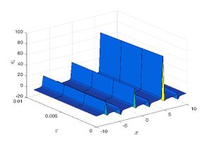
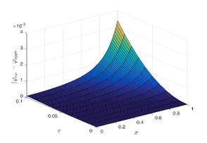
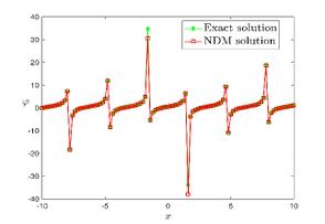
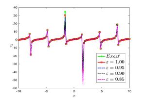
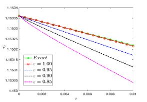
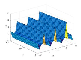
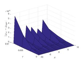
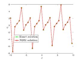
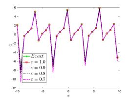
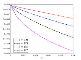
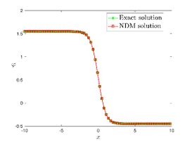
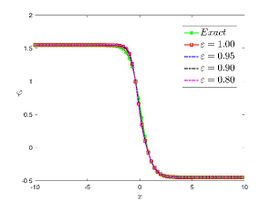
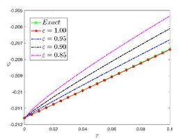
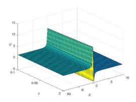
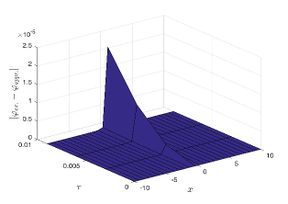
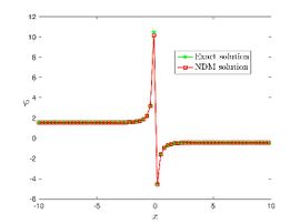
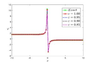
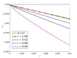
+The exact solution was compared to the second iteration of NTM in both two and three dimensions, so as to understand the geometric behavior of our approximate solution to Eq. (29) as seen in [[#img-1|Figure 1]]. When <math display="inline">\epsilon =</math><math>1</math>, <math display="inline">\epsilon =0.95</math>, <math display="inline">\epsilon =</math><math>0.90</math> and <math display="inline">\epsilon =0.80</math>, the exact solution was also compared to the solution of NTM.
+<div id='img-1'></div>
+{| class="wikitable" style="margin: 0em auto 0.1em auto;border-collapse: collapse;width:auto;"
+|-style="background:white;"
+|align="center" |
+{|style="margin: 0em auto 0.1em auto;width:auto;"
+|+
+|-
+|style="text-align: center;padding:10px;"| [[Image:Draft_Hagag_764733008-image1.jpeg|294px]]
+|style="text-align: center;padding:10px;"| [[Image:Draft_Hagag_764733008-image2.jpeg|288px]]
+|-
+|style="text-align: center;font-size: 75%;padding-bottom:10px;"|(a) 3D graph of the exact solution
+|style="text-align: center;font-size: 75%;padding-bottom:10px;"|(b) 3D graph of the NDM solution
+|-
+|style="text-align: center;padding:10px;"| [[Image:Draft_Hagag_764733008-image3.jpeg|294px]]
+|style="text-align: center;padding:10px;"| [[Image:Draft_Hagag_764733008-image4.jpeg|294px]]
+|-
+|style="text-align: center;font-size: 75%;padding-bottom:10px;"|(c) Absolute error at <math>\tau = 0.01</math>
+|style="text-align: center;font-size: 75%;padding-bottom:10px;"|(d) Graphical representation at <math>\tau = 0.01</math>
+|-
+|style="text-align: center;padding:10px;"| [[Image:Draft_Hagag_764733008-image5.jpeg|294px]]
+|style="text-align: center;padding:10px;"| [[Image:Draft_Hagag_764733008-image6.jpeg|294px]]
+|-
+|style="text-align: center;font-size: 75%;padding-bottom:10px;"|(e) Graphical representation for various values of <math>\varepsilon</math>
+|style="text-align: center;font-size: 75%;padding-bottom:10px;"|(f) Graphical representation <math>x = 1</math>
+|}
+|-
+| style="background:#efefef;text-align:left;padding:10px;font-size: 85%;"| '''Figure 1'''. Periodic wave analytical solutions <math display="inline">\varphi \left( x,\tau \right)</math>  of Eq. (29) with initial condition (36) at <math display="inline">\tau =</math><math>0.1</math>, <math display="inline">\alpha =10</math>, <math display="inline">\beta =</math><math>0.1</math>
+|}
-===Second triangular periodic solution ===
+====Second triangular periodic solution ====
 Consider the initial condition for Eq. (29) as follows [28]
@@ Line 593: / Line 661: @@
 {| style="text-align: center;margin:auto;width: 100%;"
 |-
-| <math>\begin{matrix}\varphi \left( x,0\right) &=&\frac{\alpha +\beta }{2\alpha }-\frac{1}{\alpha }cot\left( x\right) .\end{matrix}</math>
+| <math>\varphi \left( x,0\right) =\frac{\alpha +\beta }{2\alpha }-\frac{1}{\alpha }cot\left( x\right) .</math>
 |}
 |  style="text-align: center;width: 5px;text-align: right;white-space: nowrap;"|(41)
 |}
 With the above initial condition, we can get the solution of Eq. (29) employing the NDM method as follows
@@ Line 615: / Line 684: @@
 {| style="text-align: center;margin:auto;width: 100%;"
 |-
-| <math>\begin{matrix}{\varphi }_{3}&=&\frac{{\beta }^{2}{\tau }^{3\epsilon }{csc}^{4}\left( x\right) \left( 4\Gamma \left( 2\epsilon +1\right) cot\left( x\right) -2\Gamma {\left( \epsilon +1\right) }^{2}\left( \beta \left( cos\left( 2x\right) +2\right) +4cot\left( x\right) \right) \right) }{\alpha \Gamma {\left( \epsilon +1\right) }^{2}\Gamma \left( 3\epsilon +1\right) },\cdots \end{matrix}</math>
+| <math>{\varphi }_{3}=\frac{{\beta }^{2}{\tau }^{3\epsilon }{csc}^{4}\left( x\right) \left( 4\Gamma \left( 2\epsilon +1\right) cot\left( x\right) -2\Gamma {\left( \epsilon +1\right) }^{2}\left( \beta \left( cos\left( 2x\right) +2\right) +4cot\left( x\right) \right) \right) }{\alpha \Gamma {\left( \epsilon +1\right) }^{2}\Gamma \left( 3\epsilon +1\right) },\cdots </math>
 |}
 |  style="text-align: center;width: 5px;text-align: right;white-space: nowrap;"|(43)
 |}
 The above approximate results lead to the precise result shown below [28]
@@ Line 627: / Line 697: @@
 {| style="text-align: center;margin:auto;width: 100%;"
 |-
-| <math>\begin{matrix}\varphi \left( x,\tau \right) &=&\frac{\alpha +\beta }{2\alpha }-\frac{1}{\alpha }cot\left( x-\beta \tau \right).\end{matrix}</math>
+| <math>\varphi \left( x,\tau \right) =\frac{\alpha +\beta }{2\alpha }-\frac{1}{\alpha }cot\left( x-\beta \tau \right).</math>
 |}
 |  style="text-align: center;width: 5px;text-align: right;white-space: nowrap;"|(44)
 |}
-The approximate solutions and Table 2 demonstrate that the precise solution of Eq. (29) has a generic type that corresponds to the analytical solutions listed above when <math display="inline">\epsilon =</math><math>1</math>.
+The approximate solutions and [[#tab-2|Table 2]] demonstrate that the precise solution of Eq. (29) has a generic type that corresponds to the analytical solutions listed above when <math display="inline">\epsilon =</math><math>1</math>.
-<span id='first-multiple-soliton-like-solution'></span>
+<div class="center" style="font-size: 75%;">'''Table 2'''. Comparison of the NDM solution and exact solution for case 2 at <math display="inline">\tau =</math><math>0.1</math>, <math display="inline">\alpha =10</math>, <math display="inline">\beta =</math><math>0.1</math></div>
-===First multiple soliton-like solution ===
+<div id='tab-2'></div>
+{| class="wikitable" style="margin: 1em auto 0.1em auto;border-collapse: collapse;font-size:85%;width:auto;"
+|-style="text-align:center"
+! <math>x</math> !! <math>{\varphi }_{Ex}</math> !! <math>{\varphi }_{NDM}</math> !! E !! <math>\epsilon =0.95</math> !! <math>\epsilon =0.90</math>
+|-
+|  style="text-align: center;"|0.1
+|  style="text-align: center;"|-0.603109
+|  style="text-align: center;"|-0.602998
+|  style="text-align: center;"|1.1111E-04
+|  style="text-align: center;"|-0.633041
+|  style="text-align: center;"|-0.680789
+|-
+|  style="text-align: center;"|0.3
+|  style="text-align: center;"|0.169894
+|  style="text-align: center;"|0.169894
+|  style="text-align: center;"|4.2571E-07
+|  style="text-align: center;"|0.168038
+|  style="text-align: center;"|0.165851
+|-
+|  style="text-align: center;"|0.5
+|  style="text-align: center;"|0.317519
+|  style="text-align: center;"|0.317519
+|  style="text-align: center;"|3.2646E-08
+|  style="text-align: center;"|0.316853
+|  style="text-align: center;"|0.316089
+|-
+|  style="text-align: center;"|0.7
+|  style="text-align: center;"|0.383837
+|  style="text-align: center;"|0.383837
+|  style="text-align: center;"|6.0257E-09
+|  style="text-align: center;"|0.383476
+|  style="text-align: center;"|0.383064
+|-
+|  style="text-align: center;"|0.9
+|  style="text-align: center;"|0.424002
+|  style="text-align: center;"|0.424002
+|  style="text-align: center;"|1.6956E-09
+|  style="text-align: center;"|0.423760
+|  style="text-align: center;"|0.423486
+|-
+|  style="text-align: center;"|1.0
+|  style="text-align: center;"|0.439369
+|  style="text-align: center;"|0.439369
+|  style="text-align: center;"|9.8861E-10
+|  style="text-align: center;"|0.439161
+|  style="text-align: center;"|0.438924
+|}
+====First multiple soliton-like solution====
 Consider the initial condition for Eq. (29) as follows [28]
@@ Line 644: / Line 762: @@
 {| style="text-align: center;margin:auto;width: 100%;"
 |-
-| <math>\begin{matrix}\varphi \left( x,0\right) &=&\frac{\alpha +\beta }{2\alpha }-\frac{1}{\alpha }tanh\left( x\right) .\end{matrix}</math>
+| <math>\varphi \left( x,0\right) =\frac{\alpha +\beta }{2\alpha }-\frac{1}{\alpha }tanh\left( x\right) .</math>
 |}
 |  style="text-align: center;width: 5px;text-align: right;white-space: nowrap;"|(45)
 |}
-With the above initial condition, we can get the solution of Eq. (29) employing the NDM method as follows
+With the above initial condition, we can get the solution of Eq. (29) employing the NDM method as follows:
 {| class="formulaSCP" style="width: 100%;border-collapse: collapse;width: 100%;text-align: center;"
 |-
@@ Line 665: / Line 785: @@
 {| style="text-align: center;margin:auto;width: 100%;"
 |-
-| <math>\begin{matrix}{\varphi }_{3}&=&\frac{{\beta }^{2}{\tau }^{3\epsilon }{sech}^{5}\left( x\right) \left( \Gamma {\left( \epsilon +1\right) }^{2}\left( -3\beta cosh\left( x\right) +\beta cosh\left( 3x\right) -8sinh\left( x\right) \right) +4\Gamma \left( 2\epsilon +1\right) sinh\left( x\right) \right) }{\alpha \Gamma {\left( \epsilon +1\right) }^{2}\Gamma \left( 3\epsilon +1\right) },\cdots \end{matrix}</math>
+| <math>{\varphi }_{3}=\frac{{\beta }^{2}{\tau }^{3\epsilon }{sech}^{5}\left( x\right) \left( \Gamma {\left( \epsilon +1\right) }^{2}\left( -3\beta cosh\left( x\right) +\beta cosh\left( 3x\right) -8sinh\left( x\right) \right) +4\Gamma \left( 2\epsilon +1\right) sinh\left( x\right) \right) }{\alpha \Gamma {\left( \epsilon +1\right) }^{2}\Gamma \left( 3\epsilon +1\right) },\cdots </math>
 |}
 |  style="text-align: center;width: 5px;text-align: right;white-space: nowrap;"|(47)
 |}
 The above approximate results lead to the precise result shown below [28]
@@ Line 676: / Line 797: @@
 {| style="text-align: center;margin:auto;width: 100%;"
 |-
-| <math>\begin{matrix}\varphi \left( x,\tau \right) &=&\frac{\alpha +\beta }{2\alpha }-\frac{1}{\alpha }tanh\left( x-\beta \tau \right) .\end{matrix}</math>
+| <math>\varphi \left( x,\tau \right) =\frac{\alpha +\beta }{2\alpha }-\frac{1}{\alpha }tanh\left( x-\beta \tau \right) .</math>
 |}
 |  style="text-align: center;width: 5px;text-align: right;white-space: nowrap;"|(48)
 |}
-The approximate solutions and Table 1 demonstrate that the precise solution of Eq. (29) has a generic type that corresponds to the analytical solutions listed above when <math display="inline">\epsilon =</math><math>1</math>.
+The approximate solutions and [[#tab-1|Table 1]] demonstrate that the precise solution of Eq. (29) has a generic type that corresponds to the analytical solutions listed above when <math display="inline">\epsilon =1</math>.
-<span id='second-multiple-soliton-like-solution'></span>
+====Second multiple soliton-like solution====
-===Second multiple soliton-like solution===
 Consider the initial condition for Eq. (29) as follows [28]
 {| class="formulaSCP" style="width: 100%;border-collapse: collapse;width: 100%;text-align: center;"
 |-
@@ Line 693: / Line 813: @@
 {| style="text-align: center;margin:auto;width: 100%;"
 |-
-| <math>\begin{matrix}\varphi \left( x,0\right) &=&\frac{\alpha +\beta }{2\alpha }-\frac{1}{\alpha }coth\left( x\right) .\end{matrix}</math>
+| <math>\varphi \left( x,0\right) =\frac{\alpha +\beta }{2\alpha }-\frac{1}{\alpha }coth\left( x\right) .</math>
 |}
 |  style="text-align: center;width: 5px;text-align: right;white-space: nowrap;"|(49)
 |}
 With the above initial condition, we can get the solution of Eq. (29) employing the NDM method as follows
 {| class="formulaSCP" style="width: 100%;border-collapse: collapse;width: 100%;text-align: center;"
 |-
@@ Line 714: / Line 836: @@
 {| style="text-align: center;margin:auto;width: 100%;"
 |-
-| <math>\begin{matrix}{\varphi }_{3}&=&\frac{{\beta }^{2}{\tau }^{3\epsilon }{csch}^{4}\left( x\right) \left( 4\Gamma \left( 2\epsilon +1\right) coth\left( x\right) -2\Gamma {\left( \epsilon +1\right) }^{2}\left( \beta \left( cosh\left( 2x\right) +2\right) +4coth\left( x\right) \right) \right) }{\alpha \Gamma {\left( \epsilon +1\right) }^{2}\Gamma \left( 3\epsilon +1\right) },\cdots \end{matrix}</math>
+| <math>{\varphi }_{3}=\frac{{\beta }^{2}{\tau }^{3\epsilon }{csch}^{4}\left( x\right) \left( 4\Gamma \left( 2\epsilon +1\right) coth\left( x\right) -2\Gamma {\left( \epsilon +1\right) }^{2}\left( \beta \left( cosh\left( 2x\right) +2\right) +4coth\left( x\right) \right) \right) }{\alpha \Gamma {\left( \epsilon +1\right) }^{2}\Gamma \left( 3\epsilon +1\right) },\cdots </math>
 |}
 |  style="text-align: center;width: 5px;text-align: right;white-space: nowrap;"|(51)
 |}
 The above approximate results lead to the precise result shown below [28]
 {| class="formulaSCP" style="width: 100%;border-collapse: collapse;width: 100%;text-align: center;"
 |-
@@ Line 725: / Line 849: @@
 {| style="text-align: center;margin:auto;width: 100%;"
 |-
-| <math>\begin{matrix}\varphi \left( x,\tau \right) &=&\frac{\alpha +\beta }{2\alpha }-\frac{1}{\alpha }coth\left( x-\beta \tau \right) .\end{matrix}</math>
+| <math>\varphi \left( x,\tau \right) =\frac{\alpha +\beta }{2\alpha }-\frac{1}{\alpha }coth\left( x-\beta \tau \right) .</math>
 |}
 |  style="text-align: center;width: 5px;text-align: right;white-space: nowrap;"|(52)
 |}
-The approximate solutions and Table 2 demonstrate that the precise solution of Eq. (29) has a generic type that corresponds to the analytical solutions listed above when <math display="inline">\epsilon =</math><math>1</math>.
-<span id='numerical-results-and-discussion'></span>
+The approximate solutions and [[#tab-2|Table 2]] demonstrate that the precise solution of Eq. (29) has a generic type that corresponds to the analytical solutions listed above when <math display="inline">\epsilon =</math><math>1</math>.
-==6 Numerical results and discussion==
+==6. Numerical results and discussion==
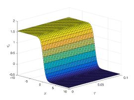
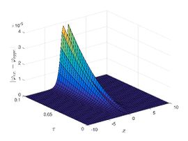
-For different choices of space and time variables, we conduct numerical simulations for fractional clannish random walker’s parabolic equation of arbitrary order. Tables 1 and 2 show the results of a numerical simulation with different values  <math display="inline">x</math> for the initial conditions considered in the first triangular periodic solution and the first multiple soliton-like solution. Similarly, the numerical analysis was carried out for the initial conditions considered in the second triangular periodic solution and the second multiple soliton-like solution, as shown in Tables 3 and 4. Some values for the four cases are also mentioned in Tables 1-4 at <math display="inline">\epsilon =</math><math>0.95</math> and <math display="inline">\epsilon =0.90</math>. We can deduce from the provided tables that the results generated by FNDM are very accurate. Figures 1a, b, 2a, b, 3a, b, 4a and b show the behavior of the exact solutions and the NDM solution for four cases. Figures 1c, 2c, 3c and 4c depict the type of absolute errors for the related equation. Figures 1d, 2d, 3d and 4d depict the graphical representation between exact and NDM solutions for four cases at <math display="inline">\tau =</math><math>0.01</math>. The response of acquired solutions with different values of <math display="inline">\epsilon</math>  between <math display="inline">\varphi \left( x,\tau \right)</math>  and <math display="inline">x</math> is presented in Figures 1e, 2e, 3e and 4e. The response of acquired solutions with different values of <math display="inline">\epsilon</math>  between <math display="inline">\varphi \left( x,\tau \right)</math>  and <math display="inline">\tau</math>  is presented in Figures 1f, 2f, 3f and 4f. The plots display the dependability and applicability of the predicted technique while analyzing nonlinear issues. Finally, the impact of generalizing models or issues from integer to fractional order can be seen in these plots. Furthermore, numerical simulations have been performed to demonstrate that the proposed technique is viable and effective.
+For different choices of space and time variables, we conduct numerical simulations for fractional clannish random walker’s parabolic equation of arbitrary order. [[#tab-1|Tables 1]] and [[#tab-2|2]] show the results of a numerical simulation with different values  <math display="inline">x</math> for the initial conditions considered in the first triangular periodic solution and the first multiple soliton-like solution. Similarly, the numerical analysis was carried out for the initial conditions considered in the second triangular periodic solution and the second multiple soliton-like solution, as shown in [[#tab-3|Tables 3]] and [[#tab-4|4]]. Some values for the four cases are also mentioned in [[#tab-1|Tables 1]]-[[#tab-4|4]] at <math display="inline">\epsilon =</math><math>0.95</math> and <math display="inline">\epsilon =0.90</math>. We can deduce from the provided tables that the results generated by FNDM are very accurate. [[#img-1|Figures 1]](a,b), [[#img-2|Figures 2]](a,b), [[#img-3|Figures 3]](a,b), [[#img-4|Figures 4]](a,b) show the behavior of the exact solutions and the NDM solution for four cases. [[#img-1|Figure 1]](c), [[#img-2|Figure 2]](c), [[#img-3|Figure 3]](c) and  [[#img-4|Figure 4]](c)  depict the type of absolute errors for the related equation. [[#img-1|Figure 1]](d), [[#img-2|Figure 2]](d), [[#img-3|Figure 3]](d) and  [[#img-4|Figure 4]](d) depict the graphical representation between exact and NDM solutions for four cases at <math display="inline">\tau =</math><math>0.01</math>. The response of acquired solutions with different values of <math display="inline">\epsilon</math>  between <math display="inline">\varphi \left( x,\tau \right)</math>  and <math display="inline">x</math> is presented in [[#img-1|Figure 1]](e), [[#img-2|Figure 2]](e), [[#img-3|Figure 3]](e) and  [[#img-4|Figure 4]](e). The response of acquired solutions with different values of <math display="inline">\epsilon</math>  between <math display="inline">\varphi \left( x,\tau \right)</math>  and <math display="inline">\tau</math>  is presented in [[#img-1|Figure 1]](f), [[#img-2|Figure 2]](f), [[#img-3|Figure 3]](f) and  [[#img-4|Figure 4]](f). The plots display the dependability and applicability of the predicted technique while analyzing nonlinear issues. Finally, the impact of generalizing models or issues from integer to fractional order can be seen in these plots. Furthermore, numerical simulations have been performed to demonstrate that the proposed technique is viable and effective.
+<div id='img-2'></div>
 {| class="wikitable" style="margin: 0em auto 0.1em auto;border-collapse: collapse;width:auto;"
 |-style="background:white;"
@@ Line 744: / Line 868: @@
 |+
 |-
-|  style="text-align: center;width: 50%;"|[[Image:Draft_Hagag_764733008-image1.jpeg|294px]]
+|style="text-align: center;padding:10px;"|[[Image:Draft_Hagag_764733008-image7.jpeg|270px]]
-|  style="text-align: center;width: 50%;"|[[Image:Draft_Hagag_764733008-image2.jpeg|288px]]
+|style="text-align: center;padding:10px;"|[[Image:Draft_Hagag_764733008-image8.jpeg|270px]]
 |-
-|  style="text-align: center;"|(a) 3D graph of the exact solution
+|style="text-align: center;font-size: 75%;padding-bottom:10px;"|(a) 3D graph of the exact solution
-|  style="text-align: center;"|(b) 3D graph of the NDM solution
+|style="text-align: center;font-size: 75%;padding-bottom:10px;"|(b) 3D graph of the NDM solution
 |-
-|  style="text-align: center;width: 50%;"|[[Image:Draft_Hagag_764733008-image3.jpeg|294px]]
+|style="text-align: center;padding:10px;"|[[Image:Draft_Hagag_764733008-image9.jpeg|270px]]
-|  style="text-align: center;width: 50%;"|[[Image:Draft_Hagag_764733008-image4.jpeg|294px]]
+|style="text-align:center;padding:10px;"|[[Image:Draft_Hagag_764733008-image10.jpeg|270px]]
 |-
-|  style="text-align: center;"|(c) Absolute error at τ = 0.01.
+|style="text-align: center;font-size: 75%;padding-bottom:10px;"|(c) Absolute error at <math>\tau = 0.01</math>
-|  style="text-align: center;"|(d) Graphical representation at τ =0.01.
+|style="text-align: center;font-size: 75%;padding-bottom:10px;"|(d) Graphical representation at <math>\tau = 0.01</math>
 |-
-|  style="text-align: center;width: 50%;"|[[Image:Draft_Hagag_764733008-image5.jpeg|294px]]
+|style="text-align: center;padding:10px;"|[[Image:Draft_Hagag_764733008-image11.jpeg|270px]]
-|  style="text-align: center;width: 50%;"|[[Image:Draft_Hagag_764733008-image6.jpeg|294px]]
+|style="text-align: center;padding:10px;"| [[Image:Draft_Hagag_764733008-image12.jpeg|270px]]
 |-
-|  style="text-align: center;"|(e) Graphical representation for various values of ε.
+|style="text-align: center;font-size: 75%;padding-bottom:10px;"|(e) Graphical representation for various values of <math>\varepsilon</math>
-|  style="text-align: center;"|(f) Graphical representation x = 1.
+|style="text-align: center;font-size: 75%;padding-bottom:10px;"|(f) Graphical representation <math>x = 1</math>
+|}
-|- style="text-align: center; font-size: 75%;"
+|-
-| colspan="2" | '''Figure 1:''' Periodic wave analytical solutions <math display="inline">\varphi \left( x,\tau \right)</math>  of Eq. (29) with initial condition (36) at <math display="inline">\tau =</math><math>0.1</math>, <math display="inline">\alpha =10</math>, <math display="inline">\beta =</math><math>0.1</math>.
+| style="background:#efefef;text-align:left;padding:10px;font-size: 85%;"| '''Figure 2'''. Periodic wave analytical solutions <math display="inline">\varphi \left( x,\tau \right)</math>  of Eq. (29) with initial condition (39) at <math display="inline">\tau =</math><math>0.1</math>, <math display="inline">\alpha =10</math>, <math display="inline">\beta =</math><math>0.1</math>
 |}
+<div id='img-3'></div>
 {| class="wikitable" style="margin: 0em auto 0.1em auto;border-collapse: collapse;width:auto;"
 |-style="background:white;"
@@ Line 774: / Line 898: @@
 |+
 |-
-|  style="text-align: center;width: 50%;"|[[Image:Draft_Hagag_764733008-image7.jpeg|270px]]
+|style="text-align: center;padding:10px;"|[[Image:Draft_Hagag_764733008-image13.jpeg|270px]]
-|  style="text-align: center;width: 50%;"|[[Image:Draft_Hagag_764733008-image8.jpeg|270px]]
+|style="text-align: center;padding:10px;"|[[Image:Draft_Hagag_764733008-image14.jpeg|270px]]
 |-
-|  style="text-align: center;"|(a) 3D graph of the exact solution
+|style="text-align: center;font-size: 75%;padding-bottom:10px;"|(a) 3D graph of the exact solution
-|  style="text-align: center;"|(b) 3D graph of the NDM solution
+|style="text-align: center;font-size: 75%;padding-bottom:10px;"|(b) 3D graph of the NDM solution
 |-
-|  style="text-align: center;width: 50%;"|[[Image:Draft_Hagag_764733008-image9.jpeg|270px]]
+|style="text-align: center;padding:10px;"|[[Image:Draft_Hagag_764733008-image15.jpeg|270px]]
-|  style="text-align: center;width: 50%;"|[[Image:Draft_Hagag_764733008-image10.jpeg|270px]]
+|style="text-align:center;padding:10px;"|[[Image:Draft_Hagag_764733008-image16.jpeg|270px]]
 |-
-|  style="text-align: center;"|(c) Absolute error at τ = 0.01.
+|style="text-align: center;font-size: 75%;padding-bottom:10px;"|(c) Absolute error at <math>\tau = 0.01</math>
-|  style="text-align: center;"|(d) Graphical representation at τ =0.01.
+|style="text-align: center;font-size: 75%;padding-bottom:10px;"|(d) Graphical representation at <math>\tau = 0.01</math>
 |-
-|  style="text-align: center;width: 50%;"|[[Image:Draft_Hagag_764733008-image11.jpeg|270px]]
+|style="text-align: center;padding:10px;"|[[Image:Draft_Hagag_764733008-image17.jpeg|270px]]
-|  style="text-align: center;width: 50%;"|[[Image:Draft_Hagag_764733008-image12.jpeg|270px]]
+|style="text-align: center;padding:10px;"|[[Image:Draft_Hagag_764733008-image18.jpeg|270px]]
 |-
-|  style="text-align: center;"|(e) Graphical representation for various values of ε.
+|style="text-align: center;font-size: 75%;padding-bottom:10px;"|(e) Graphical representation for various values of <math>\varepsilon</math>
-|  style="text-align: center;"|(f) Graphical representation x = 1.
+|style="text-align: center;font-size: 75%;padding-bottom:10px;"|(f) Graphical representation <math>x = 1</math>
+|}
 |-
-|  colspan='2'  style="vertical-align: top;"|Figure 2: Periodic wave analytical (NDM) solutions <math display="inline">\varphi \left( x,\tau \right)</math>  of Eq. (29) with initial condition (39) at <math display="inline">\tau =</math><math>0.1</math>, <math display="inline">\alpha =10</math>, <math display="inline">\beta =</math><math>0.1</math>.
+| style="background:#efefef;text-align:left;padding:10px;font-size: 85%;"| '''Figure 3'''. Periodic wave analytical solutions <math display="inline">\varphi \left( x,\tau \right)</math>  of Eq. (29) with initial condition (43) at <math display="inline">\tau =</math><math>0.1</math>, <math display="inline">\alpha =10</math>, <math display="inline">\beta =</math><math>0.1</math>
 |}
+<div id='img-3'></div>
 {| class="wikitable" style="margin: 0em auto 0.1em auto;border-collapse: collapse;width:auto;"
 |-style="background:white;"
@@ Line 803: / Line 928: @@
 |+
 |-
-|  style="text-align: center;width: 50%;"|[[Image:Draft_Hagag_764733008-image13.jpeg|270px]]
+|style="text-align: center;padding:10px;"|[[Image:Draft_Hagag_764733008-image19.jpeg|270px]]
-|  style="text-align: center;width: 50%;"|[[Image:Draft_Hagag_764733008-image14.jpeg|270px]]
+|style="text-align: center;padding:10px;"|[[Image:Draft_Hagag_764733008-image20.jpeg|270px]]
 |-
-|  style="text-align: center;"|(a) 3D graph of the exact solution
+|style="text-align: center;font-size: 75%;padding-bottom:10px;"|(a) 3D graph of the exact solution
-|  style="text-align: center;"|(b) 3D graph of the NDM solution
+|style="text-align: center;font-size: 75%;padding-bottom:10px;"|(b) 3D graph of the NDM solution
 |-
-|  style="text-align: center;width: 50%;"|[[Image:Draft_Hagag_764733008-image15.jpeg|270px]]
+|style="text-align: center;padding:10px;"|[[Image:Draft_Hagag_764733008-image21.jpeg|288px]]
-|  style="text-align: center;width: 50%;"|[[Image:Draft_Hagag_764733008-image16.jpeg|270px]]
+|style="text-align:center;padding:10px;"|[[Image:Draft_Hagag_764733008-image22.jpeg|270px]]
 |-
-|  style="text-align: center;"|(c) Absolute error at τ = 0.01.
+|style="text-align: center;font-size: 75%;padding-bottom:10px;"|(c) Absolute error at <math>\tau = 0.01</math>
-|  style="text-align: center;"|(d) Graphical representation at τ =0.01.
+|style="text-align: center;font-size: 75%;padding-bottom:10px;"|(d) Graphical representation at <math>\tau = 0.01</math>
 |-
-|  style="text-align: center;width: 50%;"|[[Image:Draft_Hagag_764733008-image17.jpeg|270px]]
+|style="text-align: center;padding:10px;"|[[Image:Draft_Hagag_764733008-image23.jpeg|294px]]
-|  style="text-align: center;width: 50%;"|[[Image:Draft_Hagag_764733008-image18.jpeg|270px]]
+|style="text-align: center;padding:10px;"|[[Image:Draft_Hagag_764733008-image24.jpeg|270px]]
 |-
-|  style="text-align: center;"|(e) Graphical representation for various values of ε.
+|style="text-align: center;font-size: 75%;padding-bottom:10px;"|(e) Graphical representation for various values of <math>\varepsilon</math>
-|  style="text-align: center;"|(f) Graphical representation x = 1.
+|style="text-align: center;font-size: 75%;padding-bottom:10px;"|(f) Graphical representation <math>x = 1</math>
-|-
-|  colspan='2'  style="vertical-align: top;"|Figure 3: Periodic wave analytical (NDM) solutions <math display="inline">\varphi \left( x,\tau \right)</math>  of Eq. (29) with initial condition (43) at <math display="inline">\tau =</math><math>0.1</math>, <math display="inline">\alpha =10</math>, <math display="inline">\beta =</math><math>0.1</math>.
 |}
-{| class="wikitable" style="margin: 0em auto 0.1em auto;border-collapse: collapse;width:auto;"
-|-style="background:white;"
-|align="center" |
-{|style="margin: 0em auto 0.1em auto;width:auto;"
-|+
 |-
-|  style="text-align: center;width: 50%;"|[[Image:Draft_Hagag_764733008-image19.jpeg|270px]]
+| style="background:#efefef;text-align:left;padding:10px;font-size: 85%;"| '''Figure 4'''. Periodic wave analytical solutions <math display="inline">\varphi \left( x,\tau \right)</math>  of Eq. (29) with initial condition (47) at <math display="inline">\tau =</math><math>0.1</math>, <math display="inline">\alpha =10</math>, <math display="inline">\beta =</math><math>0.1</math>
-|  style="text-align: center;width: 50%;"|[[Image:Draft_Hagag_764733008-image20.jpeg|270px]]
-|-
-|  style="text-align: center;"|(a) 3D graph of the exact solution
-|  style="text-align: center;"|(b) 3D graph of the NDM solution
-|-
-|  style="text-align: center;width: 50%;"|[[Image:Draft_Hagag_764733008-image21.jpeg|288px]]
-|  style="text-align: center;width: 50%;"|[[Image:Draft_Hagag_764733008-image22.jpeg|270px]]
-|-
-|  style="text-align: center;"|(c) Absolute error at τ = 0.01.
-|  style="text-align: center;"|(d) Graphical representation at τ =0.01.
-|-
-|  style="text-align: center;width: 50%;"|[[Image:Draft_Hagag_764733008-image23.jpeg|294px]]
-|  style="text-align: center;width: 50%;"|[[Image:Draft_Hagag_764733008-image24.jpeg|270px]]
-|-
-|  style="text-align: center;"|(e) Graphical representation for various values of ε.
-|  style="text-align: center;"|(f) Graphical representation x = 1.
-|-
-|  colspan='2'  style="vertical-align: top;"|Figure 4: Periodic wave analytical (NDM) solutions <math display="inline">\varphi \left( x,\tau \right)</math>  of Eq. (29) with initial condition (47) at <math display="inline">\tau =</math><math>0.1</math>, <math display="inline">\alpha =10</math>, <math display="inline">\beta =</math><math>0.1</math>.
 |}
-{|  class="floating_tableSCP wikitable" style="text-align: center; margin: 1em auto;min-width:50%;"
-|+ style="font-size: 75%;" |Table 1: Comparison of the NDM solution and exact solution for case 1 by numerical computations at <math display="inline">\tau =</math><math>0.1</math>, <math display="inline">\alpha =10</math>, <math display="inline">\beta =</math><math>0.1</math>.
-|-
-|  style="border: 1pt solid black;text-align: center;"|<math>x</math>
+<div class="center" style="font-size: 75%;">'''Table 3'''. Comparison of the NDM solution and exact solution for case 3 at <math display="inline">\tau =</math><math>0.1</math>, <math display="inline">\alpha =10</math>, <math display="inline">\beta =</math><math>0.1</math></div>
-|  style="border: 1pt solid black;text-align: center;"|<math>{\varphi }_{Ex}</math>
-|  style="border: 1pt solid black;text-align: center;"|<math>{\varphi }_{NDM}</math>
-|  style="border: 1pt solid black;text-align: center;"|E
-|  style="border: 1pt solid black;text-align: center;"|<math>\epsilon =0.95</math>
-|  style="border: 1pt solid black;text-align: center;"|<math>\epsilon =0.90</math>
-|-
-|  style="border: 1pt solid black;text-align: center;"|0.0
-|  style="border: 1pt solid black;text-align: center;"|0.503999
-|  style="border: 1pt solid black;text-align: center;"|0.503999
-|  style="border: 1pt solid black;text-align: center;"|1.3333E-12
-|  style="border: 1pt solid black;text-align: center;"|0.503855
-|  style="border: 1pt solid black;text-align: center;"|0.503691
-|-
-|  style="border: 1pt solid black;text-align: center;"|0.2
-|  style="border: 1pt solid black;text-align: center;"|0.524232
-|  style="border: 1pt solid black;text-align: center;"|0.524232
-|  style="border: 1pt solid black;text-align: center;"|1.4754E-10
-|  style="border: 1pt solid black;text-align: center;"|0.524082
-|  style="border: 1pt solid black;text-align: center;"|0.523912
-|-
-|  style="border: 1pt solid black;text-align: center;"|0.4
-|  style="border: 1pt solid black;text-align: center;"|0.546105
-|  style="border: 1pt solid black;text-align: center;"|0.546105
-|  style="border: 1pt solid black;text-align: center;"|4.1730E-10
-|  style="border: 1pt solid black;text-align: center;"|0.545936
-|  style="border: 1pt solid black;text-align: center;"|0.545746
-|-
-|  style="border: 1pt solid black;text-align: center;"|0.6
-|  style="border: 1pt solid black;text-align: center;"|0.571956
-|  style="border: 1pt solid black;text-align: center;"|0.571956
-|  style="border: 1pt solid black;text-align: center;"|1.1277E-09
-|  style="border: 1pt solid black;text-align: center;"|0.571746
-|  style="border: 1pt solid black;text-align: center;"|0.571511
-|-
-|  style="border: 1pt solid black;text-align: center;"|0.8
-|  style="border: 1pt solid black;text-align: center;"|0.605925
-|  style="border: 1pt solid black;text-align: center;"|0.605925
-|  style="border: 1pt solid black;text-align: center;"|3.6158E-09
-|  style="border: 1pt solid black;text-align: center;"|0.605634
-|  style="border: 1pt solid black;text-align: center;"|0.605308
-|-
-|  style="border: 1pt solid black;text-align: center;"|1.0
-|  style="border: 1pt solid black;text-align: center;"|0.657368
-|  style="border: 1pt solid black;text-align: center;"|0.657368
-|  style="border: 1pt solid black;text-align: center;"|1.6212E-08
-|  style="border: 1pt solid black;text-align: center;"|0.656892
-|  style="border: 1pt solid black;text-align: center;"|0.656362
-|}
-{|  class="floating_tableSCP wikitable" style="text-align: center; margin: 1em auto;min-width:50%;"
+<div id='tab-3'></div>
-|+ style="font-size: 75%;" |Table 2: Comparison of the NDM solution and exact solution for case 2 by numerical computations at <math display="inline">\tau =</math><math>0.1</math>, <math display="inline">\alpha =10</math>, <math display="inline">\beta =</math><math>0.1</math>.
+{| class="wikitable" style="margin: 1em auto 0.1em auto;border-collapse: collapse;font-size:85%;width:auto;"
+|-style="text-align:center"
+! <math>x</math>
+|  style="text-align: center;"|<math>{\varphi }_{Ex}</math>
+|  style="text-align: center;"|<math>{\varphi }_{NDM}</math>
+|  style="text-align: center;"|E
+|  style="text-align: center;"|<math>\epsilon =0.95</math>
+|  style="text-align: center;"|<math>\epsilon =0.90</math>
 |-
-|  style="border: 1pt solid black;text-align: center;"|<math>x</math>
+|  style="text-align: center;"|0.0
-|  style="border: 1pt solid black;text-align: center;"|<math>{\varphi }_{Ex}</math>
+|  style="text-align: center;"|0.505999
-|  style="border: 1pt solid black;text-align: center;"|<math>{\varphi }_{NDM}</math>
+|  style="text-align: center;"|0.505999
-|  style="border: 1pt solid black;text-align: center;"|E
+|  style="text-align: center;"|1.3332E-12
-|  style="border: 1pt solid black;text-align: center;"|<math>\epsilon =0.95</math>
+|  style="text-align: center;"|0.506145
-|  style="border: 1pt solid black;text-align: center;"|<math>\epsilon =0.90</math>
+|  style="text-align: center;"|0.506309
 |-
-|  style="border: 1pt solid black;text-align: center;"|0.1
+|  style="text-align: center;"|0.2
-|  style="border: 1pt solid black;text-align: center;"|-0.603109
+|  style="text-align: center;"|0.486225
-|  style="border: 1pt solid black;text-align: center;"|-0.602998
+|  style="text-align: center;"|0.486225
-|  style="border: 1pt solid black;text-align: center;"|1.1111E-04
+|  style="text-align: center;"|1.1814E-10
-|  style="border: 1pt solid black;text-align: center;"|-0.633041
+|  style="text-align: center;"|0.486365
-|  style="border: 1pt solid black;text-align: center;"|-0.680789
+|  style="text-align: center;"|0.486524
 |-
-|  style="border: 1pt solid black;text-align: center;"|0.3
+|  style="text-align: center;"|0.4
-|  style="border: 1pt solid black;text-align: center;"|0.169894
+|  style="text-align: center;"|0.467864
-|  style="border: 1pt solid black;text-align: center;"|0.169894
+|  style="text-align: center;"|0.467864
-|  style="border: 1pt solid black;text-align: center;"|4.2571E-07
+|  style="text-align: center;"|1.6971E-10
-|  style="border: 1pt solid black;text-align: center;"|0.168038
+|  style="text-align: center;"|0.467989
-|  style="border: 1pt solid black;text-align: center;"|0.165851
+|  style="text-align: center;"|0.468131
 |-
-|  style="border: 1pt solid black;text-align: center;"|0.5
+|  style="text-align: center;"|0.6
-|  style="border: 1pt solid black;text-align: center;"|0.317519
+|  style="text-align: center;"|0.452010
-|  style="border: 1pt solid black;text-align: center;"|0.317519
+|  style="text-align: center;"|0.452010
-|  style="border: 1pt solid black;text-align: center;"|3.2646E-08
+|  style="text-align: center;"|1.4505E-10
-|  style="border: 1pt solid black;text-align: center;"|0.316853
+|  style="text-align: center;"|0.452115
-|  style="border: 1pt solid black;text-align: center;"|0.316089
+|  style=";text-align: center;"|0.452234
 |-
-|  style="border: 1pt solid black;text-align: center;"|0.7
+|  style="text-align: center;"|0.8
-|  style="border: 1pt solid black;text-align: center;"|0.383837
+|  style="text-align: center;"|0.439159
-|  style="border: 1pt solid black;text-align: center;"|0.383837
+|  style="text-align: center;"|0.439159
-|  style="border: 1pt solid black;text-align: center;"|6.0257E-09
+|  style="text-align: center;"|8.4428E-11
-|  style="border: 1pt solid black;text-align: center;"|0.383476
+|  style="text-align: center;"|0.439242
-|  style="border: 1pt solid black;text-align: center;"|0.383064
+|  style="text-align: center;"|0.439335
 |-
-|  style="border: 1pt solid black;text-align: center;"|0.9
+|  style="text-align: center;"|1.0
-|  style="border: 1pt solid black;text-align: center;"|0.424002
+|  style="text-align: center;"|0.429264
-|  style="border: 1pt solid black;text-align: center;"|0.424002
+|  style="text-align: center;"|0.429264
-|  style="border: 1pt solid black;text-align: center;"|1.6956E-09
+|  style="text-align: center;"|2.8177E-11
-|  style="border: 1pt solid black;text-align: center;"|0.423760
+|  style="text-align: center;"|0.429326
-|  style="border: 1pt solid black;text-align: center;"|0.423486
+|  style="text-align: center;"|0.429396
-|-
-|  style="border: 1pt solid black;text-align: center;"|1.0
-|  style="border: 1pt solid black;text-align: center;"|0.439369
-|  style="border: 1pt solid black;text-align: center;"|0.439369
-|  style="border: 1pt solid black;text-align: center;"|9.8861E-10
-|  style="border: 1pt solid black;text-align: center;"|0.439161
-|  style="border: 1pt solid black;text-align: center;"|0.438924
 |}
-{|  class="floating_tableSCP wikitable" style="text-align: center; margin: 1em auto;min-width:50%;"
-|+ style="font-size: 75%;" |Table 3: Comparison of the NDM solution and exact solution for case 3 by numerical computations at <math display="inline">\tau =</math><math>0.1</math>, <math display="inline">\alpha =10</math>, <math display="inline">\beta =</math><math>0.1</math>.
-|-
-|  style="border: 1pt solid black;text-align: center;"|<math>x</math>
-|  style="border: 1pt solid black;text-align: center;"|<math>{\varphi }_{Ex}</math>
-|  style="border: 1pt solid black;text-align: center;"|<math>{\varphi }_{NDM}</math>
-|  style="border: 1pt solid black;text-align: center;"|E
-|  style="border: 1pt solid black;text-align: center;"|<math>\epsilon =0.95</math>
-|  style="border: 1pt solid black;text-align: center;"|<math>\epsilon =0.90</math>
-|-
-|  style="border: 1pt solid black;text-align: center;"|0.0
-|  style="border: 1pt solid black;text-align: center;"|0.505999
-|  style="border: 1pt solid black;text-align: center;"|0.505999
-|  style="border: 1pt solid black;text-align: center;"|1.3332E-12
-|  style="border: 1pt solid black;text-align: center;"|0.506145
-|  style="border: 1pt solid black;text-align: center;"|0.506309
-|-
-|  style="border: 1pt solid black;text-align: center;"|0.2
-|  style="border: 1pt solid black;text-align: center;"|0.486225
-|  style="border: 1pt solid black;text-align: center;"|0.486225
-|  style="border: 1pt solid black;text-align: center;"|1.1814E-10
-|  style="border: 1pt solid black;text-align: center;"|0.486365
-|  style="border: 1pt solid black;text-align: center;"|0.486524
-|-
-|  style="border: 1pt solid black;text-align: center;"|0.4
-|  style="border: 1pt solid black;text-align: center;"|0.467864
-|  style="border: 1pt solid black;text-align: center;"|0.467864
-|  style="border: 1pt solid black;text-align: center;"|1.6971E-10
-|  style="border: 1pt solid black;text-align: center;"|0.467989
-|  style="border: 1pt solid black;text-align: center;"|0.468131
-|-
-|  style="border: 1pt solid black;text-align: center;"|0.6
-|  style="border: 1pt solid black;text-align: center;"|0.452010
-|  style="border: 1pt solid black;text-align: center;"|0.452010
-|  style="border: 1pt solid black;text-align: center;"|1.4505E-10
-|  style="border: 1pt solid black;text-align: center;"|0.452115
-|  style="border: 1pt solid black;text-align: center;"|0.452234
-|-
-|  style="border: 1pt solid black;text-align: center;"|0.8
-|  style="border: 1pt solid black;text-align: center;"|0.439159
-|  style="border: 1pt solid black;text-align: center;"|0.439159
-|  style="border: 1pt solid black;text-align: center;"|8.4428E-11
-|  style="border: 1pt solid black;text-align: center;"|0.439242
-|  style="border: 1pt solid black;text-align: center;"|0.439335
-|-
-|  style="border: 1pt solid black;text-align: center;"|1.0
-|  style="border: 1pt solid black;text-align: center;"|0.429264
-|  style="border: 1pt solid black;text-align: center;"|0.429264
-|  style="border: 1pt solid black;text-align: center;"|2.8177E-11
-|  style="border: 1pt solid black;text-align: center;"|0.429326
-|  style="border: 1pt solid black;text-align: center;"|0.429396
-|}
-{|  class="floating_tableSCP wikitable" style="text-align: center; margin: 1em auto;min-width:50%;"
+<div class="center" style="font-size: 75%;">'''Table 4'''. Comparison of the NDM solution and exact solution for case 4 at <math display="inline">\tau =</math><math>0.1</math>, <math display="inline">\alpha =10</math>, <math display="inline">\beta =</math><math>0.1</math></div>
-|+ style="font-size: 75%;" |Table 4: Comparison of the NDM solution and exact solution for case 4 by numerical computations at <math display="inline">\tau =</math><math>0.1</math>, <math display="inline">\alpha =10</math>, <math display="inline">\beta =</math><math>0.1</math>.
+<div id='tab-4'></div>
+{| class="wikitable" style="margin: 1em auto 0.1em auto;border-collapse: collapse;font-size:85%;width:auto;"
+|-style="text-align:center"
+! <math>x</math>
+|  style="text-align: center;"|<math>{\varphi }_{Ex}</math>
+|  style="text-align: center;"|<math>{\varphi }_{NDM}</math>
+|  style="text-align: center;"|E
+|  style="text-align: center;"|<math>\epsilon =0.95</math>
+|  style="text-align: center;"|<math>\epsilon =0.90</math>
 |-
-|  style="border: 1pt solid black;text-align: center;"|<math>x</math>
+|  style="text-align: center;"|0.1
-|  style="border: 1pt solid black;text-align: center;"|<math>{\varphi }_{Ex}</math>
+|  style="text-align: center;"|-0.609109
-|  style="border: 1pt solid black;text-align: center;"|<math>{\varphi }_{NDM}</math>
+|  style="text-align: center;"|-0.608998
-|  style="border: 1pt solid black;text-align: center;"|E
+|  style="text-align: center;"|1.1111E-4
-|  style="border: 1pt solid black;text-align: center;"|<math>\epsilon =0.95</math>
+|  style="text-align: center;"|-0.638872
-|  style="border: 1pt solid black;text-align: center;"|<math>\epsilon =0.90</math>
+|  style="text-align: center;"|-0.686344
 |-
-|  style="border: 1pt solid black;text-align: center;"|0.1
+|  style="text-align: center;"|0.3
-|  style="border: 1pt solid black;text-align: center;"|-0.609109
+|  style="text-align: center;"|0.150560
-|  style="border: 1pt solid black;text-align: center;"|-0.608998
+|  style="text-align: center;"|0.150560
-|  style="border: 1pt solid black;text-align: center;"|1.1111E-4
+|  style="text-align: center;"|4.2571E-7
-|  style="border: 1pt solid black;text-align: center;"|-0.638872
+|  style="text-align: center;"|0.148803
-|  style="border: 1pt solid black;text-align: center;"|-0.686344
+|  style="text-align: center;"|0.146732
 |-
-|  style="border: 1pt solid black;text-align: center;"|0.3
+|  style="text-align: center;"|0.5
-|  style="border: 1pt solid black;text-align: center;"|0.150560
+|  style="text-align: center;"|0.284841
-|  style="border: 1pt solid black;text-align: center;"|0.150560
+|  style="text-align: center;"|0.284841
-|  style="border: 1pt solid black;text-align: center;"|4.2571E-7
+|  style="text-align: center;"|3.2657E-8
-|  style="border: 1pt solid black;text-align: center;"|0.148803
+|  style="text-align: center;"|0.284272
-|  style="border: 1pt solid black;text-align: center;"|0.146732
+|  style="text-align: center;"|0.283618
 |-
-|  style="border: 1pt solid black;text-align: center;"|0.5
+|  style="text-align: center;"|0.7
-|  style="border: 1pt solid black;text-align: center;"|0.284841
+|  style="text-align: center;"|0.337771
-|  style="border: 1pt solid black;text-align: center;"|0.284841
+|  style="text-align: center;"|0.337771
-|  style="border: 1pt solid black;text-align: center;"|3.2657E-8
+|  style="text-align: center;"|6.0413E-9
-|  style="border: 1pt solid black;text-align: center;"|0.284272
+|  style="text-align: center;"|0.337507
-|  style="border: 1pt solid black;text-align: center;"|0.283618
+|  style="text-align: center;"|0.337206
 |-
-|  style="border: 1pt solid black;text-align: center;"|0.7
+|  style="text-align: center;"|0.9
-|  style="border: 1pt solid black;text-align: center;"|0.337771
+|  style="text-align: center;"|0.364431
-|  style="border: 1pt solid black;text-align: center;"|0.337771
+|  style="text-align: center;"|0.364431
-|  style="border: 1pt solid black;text-align: center;"|6.0413E-9
+|  style="text-align: center;"|1.7179E-9
-|  style="border: 1pt solid black;text-align: center;"|0.337507
+|  style="text-align: center;"|0.364288
-|  style="border: 1pt solid black;text-align: center;"|0.337206
+|  style="text-align: center;"|0.364125
 |-
-|  style="border: 1pt solid black;text-align: center;"|0.9
+|  style="text-align: center;"|1.0
-|  style="border: 1pt solid black;text-align: center;"|0.364431
+|  style="text-align: center;"|0.372963
-|  style="border: 1pt solid black;text-align: center;"|0.364431
+|  style="text-align: center;"|0.372963
-|  style="border: 1pt solid black;text-align: center;"|1.7179E-9
+|  style="text-align: center;"|1.0153E-9
-|  style="border: 1pt solid black;text-align: center;"|0.364288
+|  style="text-align: center;"|0.372854
-|  style="border: 1pt solid black;text-align: center;"|0.364125
+|  style="text-align: center;"|0.372730
-|-
-|  style="border: 1pt solid black;text-align: center;"|1.0
-|  style="border: 1pt solid black;text-align: center;"|0.372963
-|  style="border: 1pt solid black;text-align: center;"|0.372963
-|  style="border: 1pt solid black;text-align: center;"|1.0153E-9
-|  style="border: 1pt solid black;text-align: center;"|0.372854
-|  style="border: 1pt solid black;text-align: center;"|0.372730
 |}
+==7. Conclusion==
-<span id='conclusion'></span>
-==7 Conclusion==
 Using innovative approaches to study and explore nonlinear physical models has always helped us grow in science and technology. We employed NDM in the present framework to analyze the fractional clannish random walker’s parabolic (CRWP) equation with fractional order. The uniqueness theorem and convergence analysis of the expected issue is investigated using Banach’s fixed-point theory. Four instances are shown to demonstrate the expected method’s reliability and applicability. For highlighted fractional order, the behaviors for the acquired findings are presented in 2D, 3D graphs, and tables. These graphs help in the conclusion of the analogical model’s stimulating actions. Furthermore, NDM does not need any conversion, perturbation, or consideration of additional polynomials or parameters while solving nonlinear problems. Examining these types of happenings can lead to new ways of looking into more real-world events. It may also inspire ideas on how to evaluate nonlinear models in science and technology using an accurate method. This paper clarifies the suggested model, which is heavily reliant on temporal instants and their histories and can be effectively shown using fractional concepts.
-'''Conflict of Interest:'''
+'''Conflict of Interest''': The author declares that there is no conflict of interest.
-The author declares that there is no conflict of interest.
 No data were used to support this study.
@@ Line 1,083: / Line 1,076: @@
 ==References==
-[1] Miller, K.S. and Ross, B., 1993. An introduction to the fractional calculus and fractional differential equations.
+<div class="auto" style="text-align: left;width: auto; margin-left: auto; margin-right: auto;font-size: 85%;">
-[2] Kilbas, A.A., Srivastava, H.M. and Trujillo, J.J., 2006. Theory and applications of fractional differential equations (Vol. 204). elsevier.
+[1] Miller K.S.,  Ross B. An introduction to the fractional calculus and fractional differential equations.  Wiley-Interscience, 1st edition, pp. 384, 1993.
-[3] Kilbas, A.A., Marichev, O.I. and Samko, S.G., 1993. Fractional integrals and derivatives (theory and applications).
+[2] Kilbas A.A., Srivastava H.M.,  Trujillo J.J. Theory and applications of fractional differential equations. Elsevier, Vol. 204, pp. 523, 2006.
-[4] Herzallah, M.A., Muslih, S.I., Baleanu, D. and Rabei, E.M., 2011. Hamilton–Jacobi and fractional like action with time scaling. Nonlinear Dynamics, 66, pp.549-555.
+[3] Samko S.G., Kilbas A.A., Marichev O.I.   Fractional integrals and derivatives: Theory and applications.  Gordon and Breach Science Publishers,  pp. 976, 1993.
-[5] West, B.J., Bologna, M., Grigolini, P., West, B.J., Bologna, M. and Grigolini, P., 2003. Fractional laplace transforms. Physics of Fractal Operators, pp.157-183.
+[4] Herzallah M.A., Muslih S.I., Baleanu D., Rabei E.M. Hamilton–Jacobi and fractional like action with time scaling. Nonlinear Dynamics, 66:549-555, 2011.
-[6] Alqahtani, Z., & Hagag, A. E. (2023). A fractional numerical study on a plant disease model with replanting and preventive treatment. Métodos numéricos para cálculo y diseño en ingeniería: Revista internacional, 39(3), 1-21.
+[5] West B.J., Bologna M., Grigolini P., West B.J., Bologna M., Grigolini P. Fractional laplace transforms. Physics of Fractal Operators, pp. 157-183, 2003.
-[7] Jesus, I.S. and Tenreiro Machado, J.A., 2008. Fractional control of heat diffusion systems. Nonlinear dynamics, 54, pp.263-282.
+[6] Alqahtani, Z. and Hagag, A.E. A fractional numerical study on a plant disease model with replanting and preventive treatment. Métodos numéricos para cálculo y diseño en ingeniería: Revista internacional, 39(3):1-21, 2023.
-[8] Feng, Z., 2002. The first-integral method to study the Burgers–Korteweg–de Vries equation. Journal of Physics A: Mathematical and General, 35(2), p.343.
+[7] Alqahtani, Z. and Hagag, A.E. A new semi-analytical solution of compound KdV-Burgers equation of fractional order. Métodos numéricos para cálculo y diseño en ingeniería: Revista internacional, 39(4):1-16, 2023.
-[9] Ege, S.M. and Misirli, E., 2014. The modified Kudryashov method for solving some fractional-order nonlinear equations. Advances in Difference Equations, 2014, pp.1-13.
+[8] Feng Z. The first-integral method to study the Burgers–Korteweg–de Vries equation. Journal of Physics A: Mathematical and General, 35(2):343, 2002.
-[10] Kaplan, M., Bekir, A. and Akbulut, A., 2016. A generalized Kudryashov method to some nonlinear evolution equations in mathematical physics. Nonlinear Dynamics, 85, pp.2843-2850.
+[9] Ege S.M., Misirli E. The modified Kudryashov method for solving some fractional-order nonlinear equations. Advances in Difference Equations, 2014:1-13, 2014.
-[11] Ma, W.X., Wu, H. and He, J., 2007. Partial differential equations possessing Frobenius integrable decompositions. Physics Letters A, 364(1), pp.29-32.
+[10] Kaplan M., Bekir A.,  Akbulut A. A generalized Kudryashov method to some nonlinear evolution equations in mathematical physics. Nonlinear Dynamics, 85:2843-2850, 2016.
-[12] Bekir, A. and Güner, Ö., 2014. Analytical approach for the space-time nonlinear partial differential fractional equation. International Journal of Nonlinear Sciences and Numerical Simulation, 15(7-8), pp.463-470.
+[11] Ma W.X., Wu H., He J. Partial differential equations possessing Frobenius integrable decompositions. Physics Letters A, 364(1):29-32, 2007.
-[13] Zhang, S. and Zhang, H.Q., 2011. Fractional sub-equation method and its applications to nonlinear fractional PDEs. Physics Letters A, 375(7), pp.1069-1073.
+[12] Bekir A.,  Güner, Ö. Analytical approach for the space-time nonlinear partial differential fractional equation. International Journal of Nonlinear Sciences and Numerical Simulation, 15(7-8):463-470, 2014.
-[14] Guo, S., Mei, L., Li, Y. and Sun, Y., 2012. The improved fractional sub-equation method and its applications to the space–time fractional differential equations in fluid mechanics. Physics Letters A, 376(4), pp.407-411.
+[13] Zhang S., Zhang H.Q. Fractional sub-equation method and its applications to nonlinear fractional PDEs. Physics Letters A, 375(7):1069-1073, 2011.
-[15] Jawad, A.J.A.M., Petković, M.D. and Biswas, A., 2010. Modified simple equation method for nonlinear evolution equations. Applied Mathematics and Computation, 217(2), pp.869-877.
+[14] Guo S., Mei L., Li Y.,  Sun Y. The improved fractional sub-equation method and its applications to the space–time fractional differential equations in fluid mechanics. Physics Letters A, 376(4):407-411, 2012.
-[16] Kilic, B., 2015. Improved šG 0/GŽ-Expansion Method for the Time-Fractional Biological Population Model and Cahn–Hilliard Equation. Journal of Computational and Nonlinear Dynamics, 10, pp.051016-1.
+[15] Jawad A.J.A.M., Petković M.D., Biswas A. Modified simple equation method for nonlinear evolution equations. Applied Mathematics and Computation, 217(2):869-877, 2010.
-[17] Kumar, D., Hosseini, K. and Samadani, F., 2017. The sine-Gordon expansion method to look for the traveling wave solutions of the Tzitzéica type equations in nonlinear optics. Optik, 149, pp.439-446.
+[16] Baleanu D., Uǧurlu Y., İnç M., Kilic B. Improved (G'/G)-expansion method for the time-fractional biological population model and Cahn–Hilliard equation. Journal of Computational and Nonlinear Dynamics, 10:051016-1, 2015.
-[18] Seadawy, A.R., Kumar, D. and Chakrabarty, A.K., 2018. Dispersive optical soliton solutions for the hyperbolic and cubic-quintic nonlinear Schrödinger equations via the extended sinh-Gordon equation expansion method. The European Physical Journal Plus, 133(5), p.182.
+[17] Kumar D., Hosseini K.,  Samadani F. The sine-Gordon expansion method to look for the traveling wave solutions of the Tzitzéica type equations in nonlinear optics. Optik, 149:439-446, 2017.
-[19] Kumar, D. and Kaplan, M., 2018. New analytical solutions of (2+ 1)-dimensional conformable time fractional Zoomeron equation via two distinct techniques. Chinese journal of physics, 56(5), pp.2173-2185.
+[18] Seadawy A.R., Kumar D.,  Chakrabarty A.K. Dispersive optical soliton solutions for the hyperbolic and cubic-quintic nonlinear Schrödinger equations via the extended sinh-Gordon equation expansion method. The European Physical Journal Plus, 133(5):182, 2018.
-[20] Chen, H. and Zhang, H., 2004. New multiple soliton solutions to the general Burgers–Fisher equation and the Kuramoto–Sivashinsky equation. Chaos, Solitons & Fractals, 19(1), pp.71-76.
+[19] Kumar D., Kaplan M. New analytical solutions of (2+1)-dimensional conformable time fractional Zoomeron equation via two distinct techniques. Chinese Journal of Physics, 56(5):2173-2185, 2018.
-[21] Adomian, G., 1984. A new approach to nonlinear partial differential equations. Journal of Mathematical Analysis and Applications, 102(2), pp.420-434.
+[20] Chen H.,  Zhang H. New multiple soliton solutions to the general Burgers–Fisher equation and the Kuramoto–Sivashinsky equation. Chaos, Solitons & Fractals, 19(1):71-76, 2004.
-[22] Sakar, M.G., Erdogan, F. and Yıldırım, A., 2012. Variational iteration method for the time-fractional Fornberg–Whitham equation. Computers & Mathematics with Applications, 63(9), pp.1382-1388.
+[21] Adomian G. A new approach to nonlinear partial differential equations. Journal of Mathematical Analysis and Applications, 102(2):420-434, 1984.
-[23] Rawashdeh, M.S. and Al-Jammal, H., 2016. New approximate solutions to fractional nonlinear systems of partial differential equations using the FNDM. Advances in Difference Equations, 2016(1), pp.1-19.
+[22] Sakar M.G., Erdogan F.,  Yıldırım A. Variational iteration method for the time-fractional Fornberg–Whitham equation. Computers & Mathematics with Applications, 63(9):1382-1388, 2012.
-[24] Rawashdeh, M.S. and Al-Jammal, H., 2016. Numerical solutions for systems of nonlinear fractional ordinary differential equations using the FNDM. Mediterranean Journal of Mathematics, 13, pp.4661-4677.
+[23] Rawashdeh M.S., Al-Jammal H. New approximate solutions to fractional nonlinear systems of partial differential equations using the FNDM. Advances in Difference Equations, 2016(1):1-19, 2016.
-[25] Debnath, L. and Debnath, L., 2005. Nonlinear partial differential equations for scientists and engineers (pp. 528-529). Boston: Birkhäuser.
+[24] Rawashdeh M.S., Al-Jammal H. Numerical solutions for systems of nonlinear fractional ordinary differential equations using the FNDM. Mediterranean Journal of Mathematics, 13:4661-4677, 2016.
-[26] Wazwaz, A.M., 2002. Partial differential equations. CRC Press.
+[25] Debnath L. Nonlinear partial differential equations for scientists and engineers. Birkhäuser Boston, MA,  pp. 738, 2005.
-[27] BULUT, H., 2013. Exact solutions for some fractional nonlinear partial differential equations via Kudryashov method. Physical Sciences, 8(1), pp.24-63.
+[26] Wazwaz A.M. Partial differential equations. CRC Press, pp. 476, 2002.
-[28] Uğurlu, Y. and Kaya, D., 2007. Analytic method for solitary solutions of some partial differential equations. Physics Letters A, 370(3-4), pp.251-259.
+[27] Bulut H. Exact solutions for some fractional nonlinear partial differential equations via Kudryashov method. Physical Sciences, 8(1):24-63, 2013.
-[29] Odabasi, M. and Misirli, E., 2018. On the solutions of the nonlinear fractional differential equations via the modified trial equation method. Mathematical Methods in the Applied Sciences, 41(3), pp.904-911.
+[28] Uğurlu Y., Kaya D. Analytic method for solitary solutions of some partial differential equations. Physics Letters A, 370(3-4):251-259, 2007.
-[30] Guner, O., Bekir, A. and Ünsal, Ö., 2016. Two reliable methods for solving the time fractional Clannish Random Walker's Parabolic equation. Optik, 127(20), pp.9571-9577.
+[29] Odabasi M., Misirli E. On the solutions of the nonlinear fractional differential equations via the modified trial equation method. Mathematical Methods in the Applied Sciences, 41(3):904-911, 2018.
-[31] Bashar, M.H., Tahseen, T. and SHAHEN, N.H., 2021. Application of the Advanced exp (-φ (ξ))-expansion method to the Nonlinear Conformable Time-Fractional Partial Differential Equations. Turkish Journal of Mathematics and Computer Science, 13(1), pp.68-80.
+[30] Guner O., Bekir A., Ünsal Ö. Two reliable methods for solving the time fractional Clannish Random Walker's Parabolic equation. Optik, 127(20):9571-9577, 2016.
-[32] Podlubny, I., 1998. Fractional differential equations: an introduction to fractional derivatives, fractional differential equations, to methods of their solution and some of their applications. Elsevier.
+[31] Bashar M.H., Tahseen T.,  Shahen N.H. Application of the advanced exp (-φ (ξ))-expansion method to the nonlinear conformable time-fractional partial differential equations. Turkish Journal of Mathematics and Computer Science, 13(1):68-80, 2021.
-[33] Mainardi, F., 1994. On the initial value problem for the fractional diffusion-wave equation. Waves and Stability in Continuous Media, World Scientific, Singapore, 1994, pp.246-251.
+[32] Podlubny I. Fractional differential equations: an introduction to fractional derivatives, fractional differential equations, to methods of their solution and some of their applications. Academic Press, Elsevier, pp. 340, 1998.
-[34] Loonker, D. and Banerji, P.K., 2013. Solution of fractional ordinary differential equations by natural transform. Int. J. Math. Eng. Sci, 12(2), pp.1-7.
+[33] Mainardi F. On the initial value problem for the fractional diffusion-wave equation.  In Rionero S. and Ruggeri T. (Eds.), Waves and Stability in Continuous Media, World Scientific, Singapore, pp.246-251, 1994.
+[34] Loonker D.,  Banerji P.K. Solution of fractional ordinary differential equations by natural transform. Int. J. Math. Eng. Sci., 12(2):1-7, 2013.
-[35] Singh, P. and Sharma, D., 2018. Convergence and error analysis of series solution of nonlinear partial differential equation. Nonlinear Engineering, 7(4), pp.303-308.
+[35] Singh P., Sharma D. Convergence and error analysis of series solution of nonlinear partial differential equation. Nonlinear Engineering, 7(4):303-308, 2018.
-[36] Kreyszig, E., 1991. Introductory functional analysis with applications (Vol. 17). John Wiley & Sons.
+[36] Kreyszig E. Introductory functional analysis with applications.  John Wiley & Sons, Vol. 17, pp. 704, 1991.