| (39 intermediate revisions by 2 users not shown) | |||
| Line 48: | Line 48: | ||
| style="text-align: center;" | <math> u(x,y,0) = g(x,y) (x, y) \in \Omega ,</math> | | style="text-align: center;" | <math> u(x,y,0) = g(x,y) (x, y) \in \Omega ,</math> | ||
|- | |- | ||
| − | | style="text-align: center;" | <math> u(x,y,t)|_{\partial \Omega } = g(x,y,t) (x, y) \in \Omega t\in [0,T], </math> | + | | style="text-align: center;" | <math> u(x,y,t)\Big|_{\partial \Omega } = g(x,y,t) (x, y) \in \Omega t\in [0,T], </math> |
|} | |} | ||
|} | |} | ||
| Line 55: | Line 55: | ||
<div id='img-1'></div> | <div id='img-1'></div> | ||
| − | {| style="text-align: center; border: 1px solid | + | {| style="text-align: center; border: 1px solid; margin: 1em auto; width: auto;max-width: auto;" |
|- | |- | ||
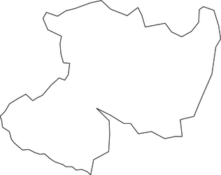
| − | + | |[[Image:Tinoco_Guerrero_et_al_2022b_9158_fig01.png|316px|Example of an Ω domain.]] | |
|- style="text-align: center; font-size: 75%;" | |- style="text-align: center; font-size: 75%;" | ||
| − | | colspan="1 | + | | colspan="1"| '''Figure 1'''. Example of an <math>\Omega </math> domain |
|} | |} | ||
| Line 104: | Line 104: | ||
|} | |} | ||
| − | where <math display="inline">\Gamma _0, \Gamma _1, \ | + | where <math display="inline">\Gamma _0, \Gamma _1, \cdots , \Gamma _q</math> are adequate weighs. |
<div id='img-2'></div> | <div id='img-2'></div> | ||
| − | {| style="text-align: center; border: 1px solid | + | {| style="text-align: center; border: 1px solid; margin: 1em auto; width: auto;max-width: auto;" |
|- | |- | ||
| − | + | |[[Image:Tinoco_Guerrero_et_al_2022b_5181_fig02.png|283px|Arbitrary distribution of p₀ and its neighbors.]] | |
|- style="text-align: center; font-size: 75%;" | |- style="text-align: center; font-size: 75%;" | ||
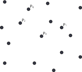
| − | | colspan="1 | + | | colspan="1" | '''Figure 2'''. Arbitrary distribution of <math>p_0</math> and its neighbors |
|} | |} | ||
| Line 138: | Line 138: | ||
{| style="text-align: left; margin:auto;width: 100%;" | {| style="text-align: left; margin:auto;width: 100%;" | ||
|- | |- | ||
| − | | style="text-align: center;" | <math>\left( \begin{array}{ | + | | style="text-align: center;" | <math>\left( \begin{array}{cccc}1 & 1 & ... & 1\\ 0 & \Delta x_1 & ... & \Delta x_q\\ 0 & \Delta y_1 & ... & \Delta y_q\\ 0 & (\Delta x_1)^2 & ... & (\Delta x_q)^2\\ 0 & \Delta x_1\Delta y_1 & ... & \Delta x_q \Delta y_q\\ 0 & (\Delta y_1)^2 & ... & (\Delta y_q)^2\\ \end{array} \right) \left( \begin{array}{c}\Gamma _0\\ \Gamma _1\\ \Gamma _2\\ \cdot\\ \cdot\\ \cdot\\ \Gamma _q\\ \end{array} \right) = \left( \begin{array}{c}F(p_0)\\ D(p_0)\\ E(p_0)\\ 2A(p_0)\\ B(p_0)\\ 2C(p_0)\\ \end{array} \right), </math> |
|} | |} | ||
| style="width: 5px;text-align: right;white-space: nowrap;" | (5) | | style="width: 5px;text-align: right;white-space: nowrap;" | (5) | ||
| Line 164: | Line 164: | ||
{| style="text-align: left; margin:auto;width: 100%;" | {| style="text-align: left; margin:auto;width: 100%;" | ||
|- | |- | ||
| − | | style="text-align: center;" | <math>\left( \begin{array}{ | + | | style="text-align: center;" | <math>\left( \begin{array}{ccc}\Delta x_1 & ... & \Delta x_q\\ \Delta y_1 & ... & \Delta y_q\\ (\Delta x_1)^2 & ... & (\Delta x_q)^2\\ \Delta x_1\Delta y_1 & ... & \Delta x_q \Delta y_q\\ (\Delta y_1)^2 & ... & (\Delta y_q)^2\\ \end{array} \right) \left( \begin{array}{c}\Gamma _1\\ \Gamma _2\\ \cdot\\ \cdot\\ \cdot\\ \Gamma _q\\ \end{array} \right) = \left( \begin{array}{c}D(p_0)\\ E(p_0)\\ 2A(p_0)\\ B(p_0)\\ 2C(p_0)\\ \end{array} \right), </math> |
|} | |} | ||
| style="width: 5px;text-align: right;white-space: nowrap;" | (7) | | style="width: 5px;text-align: right;white-space: nowrap;" | (7) | ||
|} | |} | ||
| − | can be solved using the reduced Cholesky factorization of its normal equations, as in <span id='citeF-19'></span>[[#cite-19|[19]]], namely | + | can be solved using the reduced Cholesky factorization of its normal equations, as in Tinoco-Guerrero et al. <span id='citeF-19'></span>[[#cite-19|[19]]], namely |
{| class="formulaSCP" style="width: 100%; text-align: left;" | {| class="formulaSCP" style="width: 100%; text-align: left;" | ||
| Line 187: | Line 187: | ||
{| style="text-align: left; margin:auto;width: 100%;" | {| style="text-align: left; margin:auto;width: 100%;" | ||
|- | |- | ||
| − | | style="text-align: center;" | <math> M = \left( \begin{array}{ | + | | style="text-align: center;" | <math> M = \left( \begin{array}{ccc} \Delta x_1 & ... & \Delta x_q\\ \Delta y_1 & ... & \Delta y_q\\ (\Delta x_1)^2 & ... & (\Delta x_q)^2\\ \Delta x_1\Delta y_1 & ... & \Delta x_q \Delta y_q\\ (\Delta y_1)^2 & ... & (\Delta y_q)^2\\ \end{array} \right), \quad \Gamma = \left( \begin{array}{c} \Gamma _1\\ \Gamma _2\\ \cdot\\ \cdot\\ \cdot\\ \Gamma _q\\ \end{array} \right), \quad \beta = \left( \begin{array}{c} D(p_0)\\ E(p_0)\\ 2A(p_0)\\ B(p_0)\\ 2C(p_0)\\ \end{array} \right). </math> |
|} | |} | ||
|} | |} | ||
| − | The value of <math display="inline">\Gamma _0</math> is then obtained from ([[#eq-6|6]]) assuming, for the case of the diffusion equation, <math display="inline">F(p_0) = 0</math>. | + | The value of <math display="inline">\Gamma _0</math> is then obtained from Eq.([[#eq-6|6]]) assuming, for the case of the diffusion equation, <math display="inline">F(p_0) = 0</math>. |
Now, the scheme defined by Eq.([[#eq-7|7]]) can be used to approximate the linear operator | Now, the scheme defined by Eq.([[#eq-7|7]]) can be used to approximate the linear operator | ||
| Line 222: | Line 222: | ||
<div id='img-3'></div> | <div id='img-3'></div> | ||
| − | {| style="text-align: center; border: 1px solid | + | {| style="text-align: center; border: 1px solid; margin: 1em auto; width: auto;max-width: auto;" |
|- | |- | ||
| − | + | |[[Image:Tinoco_Guerrero_et_al_2022b_6735_fig03.png|326px|Centered stencil used in the scheme.]] | |
|- style="text-align: center; font-size: 75%;" | |- style="text-align: center; font-size: 75%;" | ||
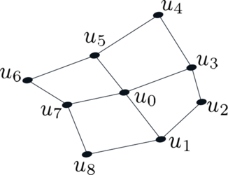
| − | | colspan="1 | + | | colspan="1" | '''Figure 3'''. Centered stencil used in the scheme |
|} | |} | ||
| − | Once a discretization of the spatial operator is obtained, following the idea presented in <span id='citeF-1'></span>[[#cite-1|[1]]], the semi-discretized PDE can be rewritten as a linear ODE system in time, | + | Once a discretization of the spatial operator is obtained, following the idea presented in Tinoco-Guerrero et al. <span id='citeF-1'></span>[[#cite-1|[1]]], the semi-discretized PDE can be rewritten as a linear ODE system in time, |
{| class="formulaSCP" style="width: 100%; text-align: left;" | {| class="formulaSCP" style="width: 100%; text-align: left;" | ||
| Line 237: | Line 237: | ||
{| style="text-align: left; margin:auto;width: 100%;" | {| style="text-align: left; margin:auto;width: 100%;" | ||
|- | |- | ||
| − | | style="text-align: center;" | <math> \frac{\partial }{\partial t}u_{i}(t) = \sum _{j=0}^{8}\Gamma _{j}u_{j}(t), i = 1,\ | + | | style="text-align: center;" | <math> \frac{\partial }{\partial t}u_{i}(t) = \sum _{j=0}^{8}\Gamma _{j}u_{j}(t), \qquad i = 1,\cdots ,m, </math> |
|} | |} | ||
|} | |} | ||
| Line 346: | Line 346: | ||
in all the cases, <math display="inline">k</math> represents the time level. | in all the cases, <math display="inline">k</math> represents the time level. | ||
| − | ==3 Numerical tests== | + | ==3. Numerical tests== |
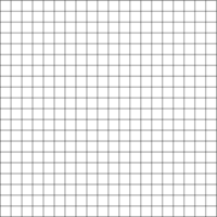
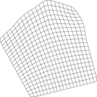
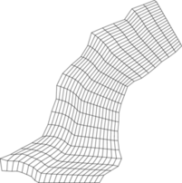
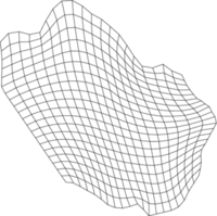
| − | To show the performance of the proposed scheme, the problem of obtaining a numerical solution to the diffusion equation in four different regions was proposed. The first region, denoted as A, corresponds to the unitary square, for comparison reasons, and the other three regions, denoted as B, C, and D, are non-rectangular planar domains. All the regions were scaled to fit on <math display="inline">[0,1]\times [0,1]</math>, and meshed with <math display="inline">21\times{21}</math> nodes, following a variational procedure implemented in UNAMalla <span id='citeF-21'></span>[[#cite-21|[21]]], then they were subdivided to obtain meshes with <math display="inline">41\times{41}</math> nodes. The meshes for with <math display="inline">21\times{21}</math> nodes for each region can be seen in | + | To show the performance of the proposed scheme, the problem of obtaining a numerical solution to the diffusion equation in four different regions was proposed. The first region, denoted as A, corresponds to the unitary square, for comparison reasons, and the other three regions, denoted as B, C, and D, are non-rectangular planar domains. All the regions were scaled to fit on <math display="inline">[0,1]\times [0,1]</math>, and meshed with <math display="inline">21\times{21}</math> nodes, following a variational procedure implemented in UNAMalla <span id='citeF-21'></span>[[#cite-21|[21]]], then they were subdivided to obtain meshes with <math display="inline">41\times{41}</math> nodes. The meshes for with <math display="inline">21\times{21}</math> nodes for each region can be seen in [[#img-4|Figure 4]]. |
<div id='img-4'></div> | <div id='img-4'></div> | ||
| − | {| | + | {| style="text-align: center; border: 1px solid #BBB; margin: 1em auto; width: auto;max-width: auto;" |
|- | |- | ||
| − | |[[Image: | + | |style="padding:10px;"| [[Image:Tinoco_Guerrero_et_al_2022b_8782_fig04a.png|200x200px]] |
| − | |[[Image: | + | |style="padding:10px;"|[[Image:Tinoco_Guerrero_et_al_2022b_4930_fig04b.png|200x200px]] |
|- | |- | ||
| − | |[[Image: | + | |style="padding:10px;"|[[Image:Tinoco_Guerrero_et_al_2022b_1349_fig04c.png|202x202px]] |
| − | |[[Image: | + | |style="padding:10px;"|[[Image:Tinoco_Guerrero_et_al_2022b_4219_fig04d.png|200x200px|Meshes of the test regions with 21×21 nodes.]] |
|- style="text-align: center; font-size: 75%;" | |- style="text-align: center; font-size: 75%;" | ||
| − | | colspan="2" | '''Figure 4 | + | | colspan="2" style="padding:10px;"| '''Figure 4.''' Meshes of the test regions with <math>21\times{21}</math> nodes |
|} | |} | ||
| + | |||
For all the regions, two different tests were performed: | For all the regions, two different tests were performed: | ||
| − | '''Test 1.''' Following the same idea as | + | '''Test 1.''' Following the same idea as in Tinoco-Ruiz <span id='citeF-22'></span>[[#cite-22|[22]]], where a well-known diffusion problem is presented, the initial and boundary conditions were taken from the closed-form solution: |
{| class="formulaSCP" style="width: 100%; text-align: left;" | {| class="formulaSCP" style="width: 100%; text-align: left;" | ||
| Line 375: | Line 376: | ||
|} | |} | ||
| − | '''Test 2.''' For comparison purposes, one of the tests presented in <span id='citeF-23'></span>[[#cite-23|[23]]], was also taken into account; in this case, the initial and boundary conditions were taken from the closed-form solution: | + | '''Test 2.''' For comparison purposes, one of the tests presented in Sánchez et al. <span id='citeF-23'></span>[[#cite-23|[23]]], was also taken into account; in this case, the initial and boundary conditions were taken from the closed-form solution: |
{| class="formulaSCP" style="width: 100%; text-align: left;" | {| class="formulaSCP" style="width: 100%; text-align: left;" | ||
| Line 412: | Line 413: | ||
where <math display="inline">U_{i,j}^k</math> and <math display="inline">u_{i,j}^k</math> are the approximated and theoretical solutions, respectively, at the <math display="inline">i,j</math>-th grid node, and <math display="inline">A_{i,j}</math> is the area of the polygon defined by the points <math display="inline">P_{i+1,j}</math>, <math display="inline">P_{i,j+1}</math>, <math display="inline">P_{i-1,j}</math> and <math display="inline">P_{i,j-1}</math>. | where <math display="inline">U_{i,j}^k</math> and <math display="inline">u_{i,j}^k</math> are the approximated and theoretical solutions, respectively, at the <math display="inline">i,j</math>-th grid node, and <math display="inline">A_{i,j}</math> is the area of the polygon defined by the points <math display="inline">P_{i+1,j}</math>, <math display="inline">P_{i,j+1}</math>, <math display="inline">P_{i-1,j}</math> and <math display="inline">P_{i,j-1}</math>. | ||
| − | + | [[#img-5|Figure 5]] presents a comparison of the numerical results obtained with the proposed scheme using the second-order Runge-Kutta approximation and the exact solutions for the test region A at time <math display="inline">t = 0.66</math>s. The approximation is presented on the left, and the exact solution on the right. | |
<div id='img-5'></div> | <div id='img-5'></div> | ||
| − | {| | + | {| style="text-align: center; border: 1px solid #BBB; margin: 1em auto; width: auto;max-width: auto;" |
|- | |- | ||
| − | |[[Image:Review_300670986669-fig13.png|716x716px]] | + | | [[Image:Review_300670986669-fig13.png|716x716px]] |
|- | |- | ||
| − | |[[Image:Review_300670986669-fig14.png|716x716px|Comparison between numerical results (left) and exact solution (right) for test region A. Test 1 (Top) and Test 2 (Bottom).]] | + | | [[Image:Review_300670986669-fig14.png|716x716px|Comparison between numerical results (left) and exact solution (right) for test region A. Test 1 (Top) and Test 2 (Bottom).]] |
|- style="text-align: center; font-size: 75%;" | |- style="text-align: center; font-size: 75%;" | ||
| − | | '''Figure 5 | + | | style="padding-bottom:10px;"|'''Figure 5'''. Comparison between numerical results (left) and exact solution (right) for test region A. Test 1 (Top) and Test 2 (Bottom) |
|} | |} | ||
| + | |||
Similarly, Figures [[#img-6|6]], [[#img-7|7]], and [[#img-8|8]] present the respective comparisons for the regions B, C, and D. | Similarly, Figures [[#img-6|6]], [[#img-7|7]], and [[#img-8|8]] present the respective comparisons for the regions B, C, and D. | ||
| − | <div id='img-6'></div> | + | <div id='img-6'></div> |
| − | {| | + | {| style="text-align: center; border: 1px solid #BBB; margin: 1em auto; width: auto;max-width: auto;" |
|- | |- | ||
|[[Image:Review_300670986669-fig15.png|716x716px]] | |[[Image:Review_300670986669-fig15.png|716x716px]] | ||
| Line 433: | Line 435: | ||
|[[Image:Review_300670986669-fig16.png|716x716px|Comparison between numerical results (left) and exact solution (right) for test region B. Test 1 (Top) and Test 2 (Bottom).]] | |[[Image:Review_300670986669-fig16.png|716x716px|Comparison between numerical results (left) and exact solution (right) for test region B. Test 1 (Top) and Test 2 (Bottom).]] | ||
|- style="text-align: center; font-size: 75%;" | |- style="text-align: center; font-size: 75%;" | ||
| − | | '''Figure 6 | + | | style="padding-bottom:10px;"|'''Figure 6'''. Comparison between numerical results (left) and exact solution (right) for test region B. Test 1 (Top) and Test 2 (Bottom) |
|} | |} | ||
| + | |||
<div id='img-7'></div> | <div id='img-7'></div> | ||
| − | {| | + | {| style="text-align: center; border: 1px solid #BBB; margin: 1em auto; width: auto;max-width: auto;" |
|- | |- | ||
|[[Image:Review_300670986669-fig17.png|716x716px]] | |[[Image:Review_300670986669-fig17.png|716x716px]] | ||
| Line 443: | Line 446: | ||
|[[Image:Review_300670986669-fig18.png|716x716px|Comparison between numerical results (left) and exact solution (right) for test region C. Test 1 (Top) and Test 2 (Bottom).]] | |[[Image:Review_300670986669-fig18.png|716x716px|Comparison between numerical results (left) and exact solution (right) for test region C. Test 1 (Top) and Test 2 (Bottom).]] | ||
|- style="text-align: center; font-size: 75%;" | |- style="text-align: center; font-size: 75%;" | ||
| − | | '''Figure 7 | + | | style="padding-bottom:10px;"|'''Figure 7'''. Comparison between numerical results (left) and exact solution (right) for test region C. Test 1 (Top) and Test 2 (Bottom) |
|} | |} | ||
| + | |||
<div id='img-8'></div> | <div id='img-8'></div> | ||
| − | {| | + | {| style="text-align: center; border: 1px solid #BBB; margin: 1em auto; width: auto;max-width: auto;" |
|- | |- | ||
|[[Image:Review_300670986669-fig19.png|716x716px]] | |[[Image:Review_300670986669-fig19.png|716x716px]] | ||
| Line 453: | Line 457: | ||
|[[Image:Review_300670986669-fig20.png|716x716px|Comparison between numerical results (left) and exact solution (right) for test region D. Test 1 (Top) and Test 2 (Bottom).]] | |[[Image:Review_300670986669-fig20.png|716x716px|Comparison between numerical results (left) and exact solution (right) for test region D. Test 1 (Top) and Test 2 (Bottom).]] | ||
|- style="text-align: center; font-size: 75%;" | |- style="text-align: center; font-size: 75%;" | ||
| − | | '''Figure 8 | + | | style="padding-bottom:10px;"|'''Figure 8'''. Comparison between numerical results (left) and exact solution (right) for test region D. Test 1 (Top) and Test 2 (Bottom) |
|} | |} | ||
| − | Figures [[#img-9|9]] to [[#img-12|12]] present the maximum value of the error <math display="inline">\| e^k\| _2</math> computed for all the regions. For each | + | |
| + | Figures [[#img-9|9]] to [[#img-12|12]] present the maximum value of the error <math display="inline">\| e^k\| _2</math> computed for all the regions. For each figure, both tests were performed in the regions meshed with <math display="inline">21\times{21}</math> nodes and <math display="inline">41\times{41}</math> nodes. | ||
<div id='img-9'></div> | <div id='img-9'></div> | ||
| − | {| | + | {| style="text-align: center; border: 1px solid #BBB; margin: 1em auto; width: auto;max-width: auto;" |
|- | |- | ||
| − | |[[Image: | + | |[[Image:Tinoco_Guerrero_et_al_2022b_3937_fig09a.png|359x359px]] |
| − | |[[Image: | + | |[[Image:Tinoco_Guerrero_et_al_2022b_6678_fig09b.png|359x359px|]] |
|- style="text-align: center; font-size: 75%;" | |- style="text-align: center; font-size: 75%;" | ||
| − | | colspan="2" | '''Figure 9 | + | | colspan="2" style="padding:10px;"| '''Figure 9'''. Maximum <math>\| e^k\| _2</math> computed for test region A with <math>21\times{21}</math> nodes (Left) and <math>41\times{41}</math> nodes (Right) |
|} | |} | ||
| + | |||
<div id='img-10'></div> | <div id='img-10'></div> | ||
| − | {| | + | {| style="text-align: center; border: 1px solid #BBB; margin: 1em auto; width: auto;max-width: auto;" |
|- | |- | ||
| − | |[[Image: | + | |[[Image:Tinoco_Guerrero_et_al_2022b_3582_fig10a.png|359px]] |
| − | |[[Image: | + | |[[Image:Tinoco_Guerrero_et_al_2022b_8582_fig10b.png|359px]] |
|- style="text-align: center; font-size: 75%;" | |- style="text-align: center; font-size: 75%;" | ||
| − | | colspan="2" | '''Figure 10 | + | | colspan="2" style="padding:10px;"| '''Figure 10'''. Maximum <math>\| e^k\| _2</math> computed for test region B with <math>21\times{21}</math> nodes (Left) and <math>41\times{41}</math> nodes (Right) |
|} | |} | ||
| + | |||
<div id='img-11'></div> | <div id='img-11'></div> | ||
| − | {| | + | {| style="text-align: center; border: 1px solid #BBB; margin: 1em auto; width: auto;max-width: auto;" |
|- | |- | ||
| − | |[[Image: | + | |[[Image:Tinoco_Guerrero_et_al_2022b_6566_fig11a.png|359px]] |
| − | |[[Image: | + | |[[Image:Tinoco_Guerrero_et_al_2022b_7935_fig11b.png|359px]] |
|- style="text-align: center; font-size: 75%;" | |- style="text-align: center; font-size: 75%;" | ||
| − | | colspan="2" | '''Figure 11 | + | | colspan="2" style="padding:10px;"| '''Figure 11'''. Maximum <math>\| e^k\| _2</math> computed for test region C with <math>21\times{21}</math> nodes (Left) and <math>41\times{41}</math> nodes (Right) |
|} | |} | ||
| + | |||
<div id='img-12'></div> | <div id='img-12'></div> | ||
| − | {| | + | {| style="text-align: center; border: 1px solid #BBB; margin: 1em auto; width: auto;max-width: auto;" |
|- | |- | ||
| − | |[[Image: | + | |[[Image:Tinoco_Guerrero_et_al_2022b_8962_fig12a.png|359px]] |
| − | |[[Image: | + | |[[Image:Tinoco_Guerrero_et_al_2022b_2351_fig12b.png|359px]] |
|- style="text-align: center; font-size: 75%;" | |- style="text-align: center; font-size: 75%;" | ||
| − | | colspan="2" | '''Figure 12 | + | | colspan="2" style="padding:10px;"| '''Figure 12'''. Maximum <math>\| e^k\| _2</math> computed for test region D with <math>21\times{21}</math> nodes (Left) and <math>41\times{41}</math> nodes (Right) |
|} | |} | ||
| − | ==4 Conclusions== | + | ==4. Conclusions== |
The numerical results show that the proposed method of Lines applied to the diffusion equation produces satisfactory numerical solutions. In the tests carried out, no spurious oscillations or instabilities were perceived. In addition, the results show that it is not necessary to “work more” by using higher Runge-Kutta methods; this scheme accomplishes better results when second-order Runge-Kutta is used to solve the Ordinary Differential Equations system. | The numerical results show that the proposed method of Lines applied to the diffusion equation produces satisfactory numerical solutions. In the tests carried out, no spurious oscillations or instabilities were perceived. In addition, the results show that it is not necessary to “work more” by using higher Runge-Kutta methods; this scheme accomplishes better results when second-order Runge-Kutta is used to solve the Ordinary Differential Equations system. | ||
| Line 504: | Line 512: | ||
* https://youtu.be/soUxe5uUY_U | * https://youtu.be/soUxe5uUY_U | ||
* https://youtu.be/479YeBjqmSs | * https://youtu.be/479YeBjqmSs | ||
| + | |||
solutions of the diffusion equation are presented on domains that are geometrical approximations of real geographical locations, where the boundary conditions are fixed as <math display="inline">0</math> and the initial condition is stated as: | solutions of the diffusion equation are presented on domains that are geometrical approximations of real geographical locations, where the boundary conditions are fixed as <math display="inline">0</math> and the initial condition is stated as: | ||
| Line 518: | Line 527: | ||
It is possible to see that even for these conditions in these regions, the scheme produces stable results that show the expected behavior. | It is possible to see that even for these conditions in these regions, the scheme produces stable results that show the expected behavior. | ||
| − | An important remark is that, even when in this work structured convex grids were used, the development of the method doesn't take into account a particular data structure, | + | An important remark is that, even when in this work structured convex grids were used, the development of the method doesn't take into account a particular data structure, i.e. this method can be used not only on structured meshes but also as a meshless method, that would be developed as future work. |
| − | == | + | ==Acknowledgments== |
We want to thank AULA CIMNE-Morelia and CIC-UMSNH for the financial support for this work. Thanks to Universidad Vasco de Quiroga for lending the facilities to perform the final part of the work done for the paper. | We want to thank AULA CIMNE-Morelia and CIC-UMSNH for the financial support for this work. Thanks to Universidad Vasco de Quiroga for lending the facilities to perform the final part of the work done for the paper. | ||
| Line 528: | Line 537: | ||
The authors would also like to thank the reviewers for their valuable feedback and suggestions to improve the present work. | The authors would also like to thank the reviewers for their valuable feedback and suggestions to improve the present work. | ||
| − | === | + | ==References== |
| + | |||
| + | <div class="auto" style="text-align: left;width: auto; margin-left: auto; margin-right: auto;font-size: 85%;"> | ||
<div id="cite-1"></div> | <div id="cite-1"></div> | ||
| − | + | [[#citeF-1|[1]]] Tinoco-Guerrero G., Domínguez-Mota F.J., Tinoco-Ruiz J.G., Lucas-Martínez J.S. Aproximación de la ecuación de advección en regiones irregulares utilizando un método de líneas y diferencias finitas generalizadas. Revista Mexicana de Métodos Numéricos, Volume 2, 3, 2028. | |
<div id="cite-2"></div> | <div id="cite-2"></div> | ||
| − | + | [[#citeF-2|[2]]] Manshoor B., Salleh H., Khalid A., Sayed Abdelaal M.A. Method of lines and Runge-Kutta method in solving partial differential equation for eeat equation. Journal of Complex Flow, 3(1):21-25, 2021. | |
<div id="cite-3"></div> | <div id="cite-3"></div> | ||
| − | + | [[#citeF-3|[3]]] Ureña Prieto F., Benito Muñoz J.J., Gavete Corvinos L. Application of the generalized finite difference method to solve the advection-diffusion equation. Journal of Computational and Applied Mathematics, 25:1849-1855, 2011. | |
<div id="cite-4"></div> | <div id="cite-4"></div> | ||
| − | + | [[#citeF-4|[4]]] Li P.-W., Fan C.-M., Grabski J.K. A meshless generalized finite difference method for solving shallow water equations with the flux limiter technique. Engineering Analysis with Boundary Elements, 131:159–173, 2021. | |
<div id="cite-5"></div> | <div id="cite-5"></div> | ||
| − | + | [[#citeF-5|[5]]] Zhang T., Lin Z.-H., Huang G.-Y., Fan C.-M., Li P.-W. Solving Boussinesq equations with a meshless finite difference method. Ocean Engineering, 198:106957, 2020. | |
<div id="cite-6"></div> | <div id="cite-6"></div> | ||
| − | + | [[#citeF-6|[6]]] Fu Z.-J., Tang Z.-C., Zhao H.-T., Li P.-W., Rabczuk T. Numerical solutions of the coupled unsteady nonlinear convection-diffusion equations based on generalized finite difference method. The European Physical Journal Plus, 134(6):1–20, 2019. | |
<div id="cite-7"></div> | <div id="cite-7"></div> | ||
| − | + | [[#citeF-7|[7]]] Zhang T., Ren Y.-F., Yang Z.-Q., Fan C.-M., Li P.-W. Application of generalized finite difference method to propagation of nonlinear water waves in numerical wave flume. Ocean Engineering, 123:278–290, 2016. | |
<div id="cite-8"></div> | <div id="cite-8"></div> | ||
| − | + | [[#citeF-8|[8]]] Li P.-W., Fan C.-M. Generalized finite difference method for two-dimensional shallow water equations. Engineering Analysis with Boundary Elements, 80:58–71, 2017. | |
<div id="cite-9"></div> | <div id="cite-9"></div> | ||
| − | + | [[#citeF-9|[9]]] Fu Z.-J., Zhang J., Li P.-W., Zheng J.-H. A semi-Lagrangian meshless framework for numerical solutions of two-dimensional sloshing phenomenon. Engineering Analysis with Boundary Elements, 112:58–67, 2020. | |
<div id="cite-10"></div> | <div id="cite-10"></div> | ||
| − | + | [[#citeF-10|[10]]] Wang Q., Kim P., Qu W. A hybrid localized meshless method for the solution of transient groundwater flow in two dimensions. Mathematics, 10(3):1-14, 2022. | |
<div id="cite-11"></div> | <div id="cite-11"></div> | ||
| − | + | [[#citeF-11|[11]]] Domínguez-Mota F.J., Mendoza-Armenta S., Tinoco-Ruiz J.G. Finite difference schemes satisfying an optimality condition. IMACS Series in Computational and Applied Mathematics: MASCOT, 2011. | |
<div id="cite-12"></div> | <div id="cite-12"></div> | ||
| − | + | [[#citeF-12|[12]]] Tinoco-Guerrero G., Domínguez-Mota F.J., Tinoco-Ruiz J.G. Numerical solution of advection equations using structured grids on plane irregular regions with a finite differences scheme. Boletín de la Sociedad Mexicana de Computación Científica y Sus Aplicaciones, 1(3):29-32, 2015. | |
<div id="cite-13"></div> | <div id="cite-13"></div> | ||
| − | + | [[#citeF-13|[13]]] Tinoco-Ruiz J.G., Domínguez-Mota F.J., Tinoco-Guerrero G., Fernández-Valdés P.M., Mendoza-Armenta S. Numerical solution of differential equations in irregular plane regions using quality structured convex grids. International Journal of Modeling, Simulation and Scientific Computing, 4(2):1340005, 2013. | |
<div id="cite-14"></div> | <div id="cite-14"></div> | ||
| − | + | [[#citeF-14|[14]]] Domínguez-Mota F.J., Lucas-Martínez J.S., Tinoco-Guerrero G. A generalized finite-differences scheme used in modeling of a direct and an inverse problem of advection-diffusion. International Journal of Applied Mathematics, 33(4):599-608, 2020. | |
<div id="cite-15"></div> | <div id="cite-15"></div> | ||
| − | + | [[#citeF-15|[15]]] Chávez-Negrete C., Domínguez-Mota F.J., Santana-Quinteros D. Numerical solution of Richards' equation of water flow by generalized finite differences. Computers and Geotechnics, 101:168–175, 2018. | |
<div id="cite-16"></div> | <div id="cite-16"></div> | ||
| − | + | [[#citeF-16|[16]]] Schiesser W. The numerical method of lines. San Diego: Academic Press, 1991. | |
<div id="cite-17"></div> | <div id="cite-17"></div> | ||
| − | + | [[#citeF-17|[17]]] Strikwerda J.C. Finite difference schemes and partial differential equations. Society for Industrial and Applied Mathematics, pp. 427, 2004. | |
<div id="cite-18"></div> | <div id="cite-18"></div> | ||
| − | + | [[#citeF-18|[18]]] Thomas J.W. Numerical partial differential equations: finite difference methods. Texts in Applied Mathematics (TAM), Volume 22, Springer, 1995. | |
<div id="cite-19"></div> | <div id="cite-19"></div> | ||
| − | + | [[#citeF-19|[19]]] Tinoco-Guerrero G., Domínguez-Mota F.J., Tinoco-Ruiz J.G. A study of the stability for a generalized finite-difference scheme applied to the advection-diffusion equation. Mathematics and Computer in Simulations, 176:301-311, 2020. | |
<div id="cite-20"></div> | <div id="cite-20"></div> | ||
| − | + | [[#citeF-20|[20]]] Butcher J.C. Conference on the numerical solution of differential equations. Lecture Notes in Mathematics (LNM), Springer, 109:133-139, 1969. | |
<div id="cite-21"></div> | <div id="cite-21"></div> | ||
| − | + | [[#citeF-21|[21]]] UNAMalla. An automatic package for numerical grid generation, 2011. | |
<div id="cite-22"></div> | <div id="cite-22"></div> | ||
| − | + | [[#citeF-22|[22]]] Tinoco-Ruiz J.G., Domínguez-Mota F.J., Tinoco-Guerrero G., Lucas-Martínez J.S. Study of the stability of a generalized finite difference scheme applied to the diffusion equation in irregular 2D space regions using convex grids. IMACS Series in Computational and Applied Mathematics: MASCOT2018, 2018. | |
<div id="cite-23"></div> | <div id="cite-23"></div> | ||
| − | + | [[#citeF-23|[23]]] Sánchez L.M., Ureña F., Benito J.J., Gavete L. Resolución de la ecuación de difusión en 2-D y 3-D utilizando diferencias finitas generalizadas. Consistencia y Estabilidad. XXI Congreso de Ecuaciones Diferenciales y Aplicaciones, Ciudad Real, pp. 1-8, 2009. | |
<div id="cite-24"></div> | <div id="cite-24"></div> | ||
| − | + | [[#citeF-24|[24]]] Abbott M.B., McCowan A.D., Warren I.R. Accuracy of short-wave numerical models. Journal of Hydraulic Engineering, 110(10):1287-1301, 1984. | |
Latest revision as of 09:34, 23 June 2022
Abstract
One of the greatest challenges in the area of applied mathematics continues to be the design of numerical methods capable of approximating the solution of partial differential equations quickly and accurately. One of the most important equations, due to the hydraulic and transport applications it has, and the large number of difficulties that it usually presents when solving it numerically is the Diffusion Equation.
In the present work, a Method of Lines applied to the numerical solution of the said equation in irregular regions is presented using a scheme of Generalized Finite Differences. The second-order finite difference method uses a central node and 8 neighbor points in order to address the spatial approximation. A series of tests and numerical results are presented, which show the accuracy of the proposed method.
Keywords: Generalized finite differences, method of lines, diffusion equation, irregular regions
1. Introduction
When a substance is been transported with a speed equal to zero, i.e. no flow moves it, then, according to the transport equation [1], the initial profile of the substance should remain the same as time goes by, maintaining the substance concentration at each point in the fluid.
However, in practice, this does not happen due to molecular diffusion; this is due to the molecules being in constant motion, causing collisions and rebounds in different directions. The molecules will tend to separate, or diffuse, within the flow. In general, this movement moves from areas with a higher density of molecules to areas with a lower density; this is called diffusion and can be described by a well-known Partial Differential Equation:
|
|
(1) |
where represents the diffusion coefficient, which tells how easy a substance diffuses in a medium.
In the past years, many people have worked in different methods to achieve good numerical solutions to this equation, involving a great variety of modern and classical techniques. Nevertheless, even though a large number of numerical methods have been proposed to solve it, a large number of these have a rather limited application to real-world scenarios since they are designed for regular regions.
This is due to the fact that the spatial discretization of the diffusion equation imposes bounds on the time step size in order to achieve numerical stability. However, the use of semidiscretization schemes allows for overcoming many stability issues by using well-known and widely used one-step methods for ordinary initial value problems. For example, in Manshoor et al. [2], a Method of Lines, involving solutions with Runge-Kutta method, is presented along with its stability analysis; the results presented show that it is possible to use this kind of method to compute numerical solutions of the equation, yet, the regions where the method is tested are unidimensional regions. On the side of the Generalized Finite Difference methods, Ureña et al. [3] present a scheme to achieve numerical solutions using this method; the results presented in this work show that it is possible to solve different Partial Differential Equations using finite differences over non-regular clouds of points; this work presents that the solutions obtained with this method satisfactorily match with the exact solution of the proposed tests. Some other authors, like Li et al. [4,5,6,7,8,9], and Wang et al. [10] have addressed a large number of applications. Nevertheless, the computational cost of the method as proposed in the aforementioned papers is high, so for each node of the cloud it is required to take up to twenty-six support nodes, even in 2D problems, which increases the computational cost of the implementation.
On the other hand, some variations of the presented generalized finite difference method for several transport equations, which produce satisfactory numerical solutions using a low-cost implementation for the spatial discretization were presented in [11,12,13,14,15]. Even though, the use of several straightforward time integration schemes remained an important issue to take into account.
For the case of interest of this work, it is important to obtain an approximation in generalized finite differences, for the spatial part, to the solution of the problem
|
|
where is a simply connected planar domain, and its boundary, and is a positively oriented Jordan polygon, as the domain shown in Figure 1.
|
| Figure 1. Example of an domain |
On the other hand, for the temporal discretization, a Method of Lines (MOL) is proposed [16]. The basic idea of the MOL is to solve a time-dependent Partial Differential Equation (PDE) by discretizing the spatial derivatives and then, integrating the semi-discretized problem as an Ordinary Differential Equations (ODE) system.
2. Proposed scheme
In order to apply a MOL for the case of the diffusion equation
|
|
it is possible to discretize the spatial derivatives applying a generalized finite differences method, for that it is convenient to considerate the approximation to the second or-er linear operator
|
|
(2) |
where , , , , , and are given functions. Within an arbitrary distribution of nodes, like the one presented in Figure 2, it is possible to approximate its value at a node using values of at some neighbor nodes , [12]. For this work, a finite difference scheme is applied at the node , which can be written as a linear combination as
|
|
(3) |
where are adequate weighs.
|
| Figure 2. Arbitrary distribution of and its neighbors |
According to Strikwerda [17] and Thomas [18], a finite difference scheme is consistent with the linear operator if the local truncation error satisfies that
|
|
(4) |
as , , , .
Using the six first terms of Taylor's series expansion, up to second order, of the consistency condition (4), it is possible to obtain the system
|
|
(5) |
where and . In order o solve this linear system, it is possible to separate the first equation of the system (5)
|
|
(6) |
and then, the problem defined by
|
|
(7) |
can be solved using the reduced Cholesky factorization of its normal equations, as in Tinoco-Guerrero et al. [19], namely
|
|
where
|
|
The value of is then obtained from Eq.(6) assuming, for the case of the diffusion equation, .
Now, the scheme defined by Eq.(7) can be used to approximate the linear operator
|
|
taking , and . The resulting coefficients, define the Finite-Difference Scheme
|
|
(8) |
for diffusion equation, where is the approximation to the solution in the point , and are the corresponding neighbor nodes of .
An important issue to be taken into account is the number of neighbors, , to use in the scheme. In this paper, 8 neighbor points were taken into account following the stencil shown in Figure 3.
|
| Figure 3. Centered stencil used in the scheme |
Once a discretization of the spatial operator is obtained, following the idea presented in Tinoco-Guerrero et al. [1], the semi-discretized PDE can be rewritten as a linear ODE system in time,
|
|
where is the total amount of grid points.
There exist several ways to approximate the solution of this ODE system, for example, it is possible to use a forward Euler method as
|
|
nevertheless, this kind of implementation has proven to be conditionally stable and, in some cases, the stability conditions are difficult to accomplish.
Another way to solve this system is the Method of Lines, where each is solved for a fixed grid node , i.e. it is solved by “lines”. As we are now dealing with a set of ODEs, it is possible to use a Runge-Kutta method, to solve the ODE on each line in order to obtain stable and accurate results.
In the present work it is proposed to use Runge-Kutta [20] of 2nd, 3rd, and 4th order, as follows.
Second-order Runge-Kutta method
|
|
where
|
|
Third-order Runge-Kutta method
|
|
where
|
|
Fourth-order Runge-Kutta method
|
|
where
|
|
in all the cases, represents the time level.
3. Numerical tests
To show the performance of the proposed scheme, the problem of obtaining a numerical solution to the diffusion equation in four different regions was proposed. The first region, denoted as A, corresponds to the unitary square, for comparison reasons, and the other three regions, denoted as B, C, and D, are non-rectangular planar domains. All the regions were scaled to fit on , and meshed with nodes, following a variational procedure implemented in UNAMalla [21], then they were subdivided to obtain meshes with nodes. The meshes for with nodes for each region can be seen in Figure 4.
|
|
|
|
| Figure 4. Meshes of the test regions with nodes | |
For all the regions, two different tests were performed:
Test 1. Following the same idea as in Tinoco-Ruiz [22], where a well-known diffusion problem is presented, the initial and boundary conditions were taken from the closed-form solution:
|
|
Test 2. For comparison purposes, one of the tests presented in Sánchez et al. [23], was also taken into account; in this case, the initial and boundary conditions were taken from the closed-form solution:
|
|
The time interval was subdivided with different discretizations, the number of time steps was chosen to satisfy the classical Courant condition [24]:
|
|
where and are the spatial steps on each grid, taken from the meshes with nodes, and .
The norm of the quadratic error, at a the time level can be computed as
|
|
where and are the approximated and theoretical solutions, respectively, at the -th grid node, and is the area of the polygon defined by the points , , and .
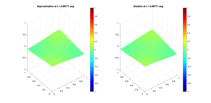
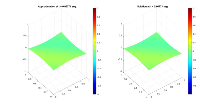
Figure 5 presents a comparison of the numerical results obtained with the proposed scheme using the second-order Runge-Kutta approximation and the exact solutions for the test region A at time s. The approximation is presented on the left, and the exact solution on the right.
|
|
| Figure 5. Comparison between numerical results (left) and exact solution (right) for test region A. Test 1 (Top) and Test 2 (Bottom) |
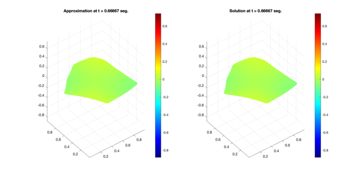
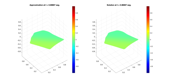
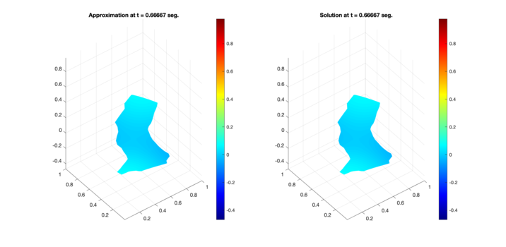
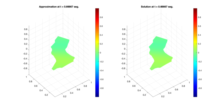
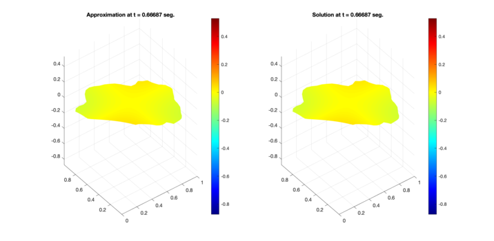
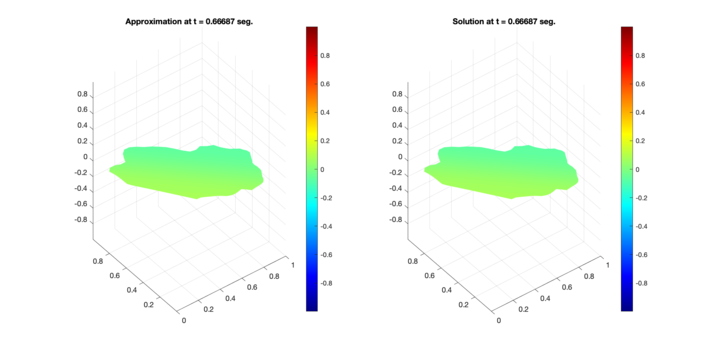
Similarly, Figures 6, 7, and 8 present the respective comparisons for the regions B, C, and D.
|
|
| Figure 6. Comparison between numerical results (left) and exact solution (right) for test region B. Test 1 (Top) and Test 2 (Bottom) |
|
|
| Figure 7. Comparison between numerical results (left) and exact solution (right) for test region C. Test 1 (Top) and Test 2 (Bottom) |
|
|
| Figure 8. Comparison between numerical results (left) and exact solution (right) for test region D. Test 1 (Top) and Test 2 (Bottom) |
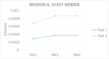
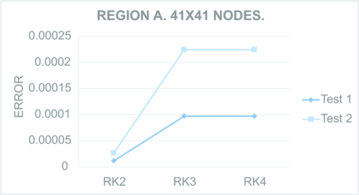
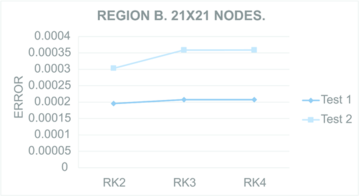
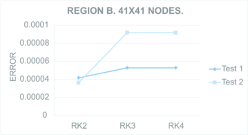
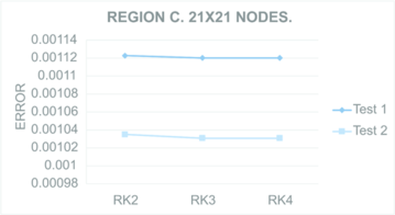
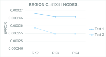
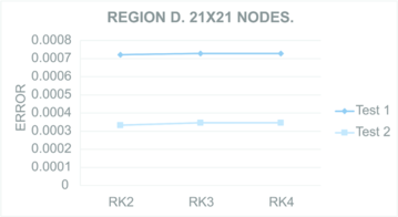
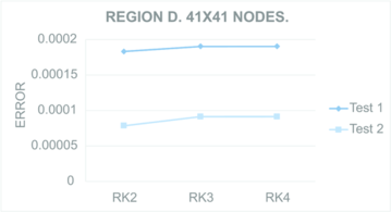
Figures 9 to 12 present the maximum value of the error computed for all the regions. For each figure, both tests were performed in the regions meshed with nodes and nodes.
|
|
| Figure 9. Maximum computed for test region A with nodes (Left) and nodes (Right) | |
|
|
| Figure 10. Maximum computed for test region B with nodes (Left) and nodes (Right) | |
|
|
| Figure 11. Maximum computed for test region C with nodes (Left) and nodes (Right) | |
|
|
| Figure 12. Maximum computed for test region D with nodes (Left) and nodes (Right) | |
4. Conclusions
The numerical results show that the proposed method of Lines applied to the diffusion equation produces satisfactory numerical solutions. In the tests carried out, no spurious oscillations or instabilities were perceived. In addition, the results show that it is not necessary to “work more” by using higher Runge-Kutta methods; this scheme accomplishes better results when second-order Runge-Kutta is used to solve the Ordinary Differential Equations system.
It is possible to appreciate that with the presented discretizations, even with the fourth-order Runge-Kutta method, acceptable numerical results can be obtained. Additionally, the numerical results shown in Figures 9 to 12 show that a refinement of the spatial mesh can improve the approximations carried out with the method; as expected in these kinds of methods. It is worth mentioning that, for all the tests, a minimum number of time steps was used, taking into account the classical theory for the diffusion equation, which makes the computational cost of this method low, since it does not require making very small temporary discretizations, as in other cases.
Furthermore, the proposed scheme can produce stable results for non-standard initial conditions in highly irregular regions. For example, in the following videos
solutions of the diffusion equation are presented on domains that are geometrical approximations of real geographical locations, where the boundary conditions are fixed as and the initial condition is stated as:
|
|
It is possible to see that even for these conditions in these regions, the scheme produces stable results that show the expected behavior.
An important remark is that, even when in this work structured convex grids were used, the development of the method doesn't take into account a particular data structure, i.e. this method can be used not only on structured meshes but also as a meshless method, that would be developed as future work.
Acknowledgments
We want to thank AULA CIMNE-Morelia and CIC-UMSNH for the financial support for this work. Thanks to Universidad Vasco de Quiroga for lending the facilities to perform the final part of the work done for the paper.
Special thanks to the ``Laboratorio de Matemáticas Aplicadas of the ``Facultad de Ciencias Físico-Matemáticas at ``Universidad Michoacana de San Nicolás de Hidalgo for lending their computational infrastructure.
The authors would also like to thank the reviewers for their valuable feedback and suggestions to improve the present work.
References
[1] Tinoco-Guerrero G., Domínguez-Mota F.J., Tinoco-Ruiz J.G., Lucas-Martínez J.S. Aproximación de la ecuación de advección en regiones irregulares utilizando un método de líneas y diferencias finitas generalizadas. Revista Mexicana de Métodos Numéricos, Volume 2, 3, 2028.
[2] Manshoor B., Salleh H., Khalid A., Sayed Abdelaal M.A. Method of lines and Runge-Kutta method in solving partial differential equation for eeat equation. Journal of Complex Flow, 3(1):21-25, 2021.
[3] Ureña Prieto F., Benito Muñoz J.J., Gavete Corvinos L. Application of the generalized finite difference method to solve the advection-diffusion equation. Journal of Computational and Applied Mathematics, 25:1849-1855, 2011.
[4] Li P.-W., Fan C.-M., Grabski J.K. A meshless generalized finite difference method for solving shallow water equations with the flux limiter technique. Engineering Analysis with Boundary Elements, 131:159–173, 2021.
[5] Zhang T., Lin Z.-H., Huang G.-Y., Fan C.-M., Li P.-W. Solving Boussinesq equations with a meshless finite difference method. Ocean Engineering, 198:106957, 2020.
[6] Fu Z.-J., Tang Z.-C., Zhao H.-T., Li P.-W., Rabczuk T. Numerical solutions of the coupled unsteady nonlinear convection-diffusion equations based on generalized finite difference method. The European Physical Journal Plus, 134(6):1–20, 2019.
[7] Zhang T., Ren Y.-F., Yang Z.-Q., Fan C.-M., Li P.-W. Application of generalized finite difference method to propagation of nonlinear water waves in numerical wave flume. Ocean Engineering, 123:278–290, 2016.
[8] Li P.-W., Fan C.-M. Generalized finite difference method for two-dimensional shallow water equations. Engineering Analysis with Boundary Elements, 80:58–71, 2017.
[9] Fu Z.-J., Zhang J., Li P.-W., Zheng J.-H. A semi-Lagrangian meshless framework for numerical solutions of two-dimensional sloshing phenomenon. Engineering Analysis with Boundary Elements, 112:58–67, 2020.
[10] Wang Q., Kim P., Qu W. A hybrid localized meshless method for the solution of transient groundwater flow in two dimensions. Mathematics, 10(3):1-14, 2022.
[11] Domínguez-Mota F.J., Mendoza-Armenta S., Tinoco-Ruiz J.G. Finite difference schemes satisfying an optimality condition. IMACS Series in Computational and Applied Mathematics: MASCOT, 2011.
[12] Tinoco-Guerrero G., Domínguez-Mota F.J., Tinoco-Ruiz J.G. Numerical solution of advection equations using structured grids on plane irregular regions with a finite differences scheme. Boletín de la Sociedad Mexicana de Computación Científica y Sus Aplicaciones, 1(3):29-32, 2015.
[13] Tinoco-Ruiz J.G., Domínguez-Mota F.J., Tinoco-Guerrero G., Fernández-Valdés P.M., Mendoza-Armenta S. Numerical solution of differential equations in irregular plane regions using quality structured convex grids. International Journal of Modeling, Simulation and Scientific Computing, 4(2):1340005, 2013.
[14] Domínguez-Mota F.J., Lucas-Martínez J.S., Tinoco-Guerrero G. A generalized finite-differences scheme used in modeling of a direct and an inverse problem of advection-diffusion. International Journal of Applied Mathematics, 33(4):599-608, 2020.
[15] Chávez-Negrete C., Domínguez-Mota F.J., Santana-Quinteros D. Numerical solution of Richards' equation of water flow by generalized finite differences. Computers and Geotechnics, 101:168–175, 2018.
[16] Schiesser W. The numerical method of lines. San Diego: Academic Press, 1991.
[17] Strikwerda J.C. Finite difference schemes and partial differential equations. Society for Industrial and Applied Mathematics, pp. 427, 2004.
[18] Thomas J.W. Numerical partial differential equations: finite difference methods. Texts in Applied Mathematics (TAM), Volume 22, Springer, 1995.
[19] Tinoco-Guerrero G., Domínguez-Mota F.J., Tinoco-Ruiz J.G. A study of the stability for a generalized finite-difference scheme applied to the advection-diffusion equation. Mathematics and Computer in Simulations, 176:301-311, 2020.
[20] Butcher J.C. Conference on the numerical solution of differential equations. Lecture Notes in Mathematics (LNM), Springer, 109:133-139, 1969.
[21] UNAMalla. An automatic package for numerical grid generation, 2011.
[22] Tinoco-Ruiz J.G., Domínguez-Mota F.J., Tinoco-Guerrero G., Lucas-Martínez J.S. Study of the stability of a generalized finite difference scheme applied to the diffusion equation in irregular 2D space regions using convex grids. IMACS Series in Computational and Applied Mathematics: MASCOT2018, 2018.
[23] Sánchez L.M., Ureña F., Benito J.J., Gavete L. Resolución de la ecuación de difusión en 2-D y 3-D utilizando diferencias finitas generalizadas. Consistencia y Estabilidad. XXI Congreso de Ecuaciones Diferenciales y Aplicaciones, Ciudad Real, pp. 1-8, 2009.
[24] Abbott M.B., McCowan A.D., Warren I.R. Accuracy of short-wave numerical models. Journal of Hydraulic Engineering, 110(10):1287-1301, 1984.Document information
Published on 14/06/22
Accepted on 07/06/22
Submitted on 19/09/21
Volume 38, Issue 2, 2022
DOI: 10.23967/j.rimni.2022.06.003
Licence: CC BY-NC-SA license