Combination of a non-local damage model for quasi-brittle materials with a mesh-adaptive finite element technique

Published in Finite Elements in Analysis and Design Vol. 112, pp. 26-39, 2016
doi: 10.1016/j.finel.2015.12.011

Abstract

Progressive fracture in quasi-brittle materials is often treated via strain softening models in continuum damage mechanics. Such constitutive relations favour spurious strain localization and ill-posedness of boundary value problems. The introduction of non-local damage models together with a characteristic length parameter controlling the size of the fracture process zone is known to regularize the problem. In order to account for the non-locality of these models, it is crucial to work with fine spatial discretizations at the damage progress zone. In this paper we present a non-local damage model in combination with a mesh-adaptive finite element technique that can help automatize the analysis of progressive fracture problems in an efficient manner. Classical two-dimensional examples are given to illustrate the presented approach.

Keywords: Quasi-brittle materials, continuum damage mechanics, non-local damage models, finite element method, mesh-adaptivity

1 Introduction

Continuum damage mechanics is a branch of continuum mechanics that describes the progressive loss of material integrity due to the propagation and coalescence of micro-cracks, micro-voids, and similar defects. These changes in the micro-structure lead to an irreversible material degradation, characterized by a loss of stiffness that can be observed on the macro-scale.

The term “continuum damage mechanics” was first used by [14], but the concept of damage was introduced by Kachanov in 1958 in the context of creep rupture [16]. In that work Kachanov introduced the concept of effective stress, and by using continuum damage he solved problems related to creep in metals. [31] gave the problem physical meaning by suggesting that the reduction of the sectional area was measured by means of the damage parameter. The thermodynamic formalism involved in the irreversible process of damage was developed by [18]. Other important contributions on damage mechanics include: [22, 33, 26, 24, 25, 8, 9], to name but a few.

The behaviour of brittle or quasi-brittle materials such as concrete, rocks, mortar or other geo-materials is particularly difficult to predict. In those cases failure is preceded by a gradual development of a non-linear fracture process zone and a localization of strain. Realistic failure analysis of such quasi-brittle structures requires the consideration of progressive damage due to micro-cracking, modelled by a constitutive law with strain softening. This typically results in highly non-linear structural responses and so efficient non-linear solvers based on arc-length control are needed for the numerical simulations [13].

If the damage parameter depends only on the strain state at the point under consideration, numerical simulations exhibit a pathological mesh dependence and the energy consumed by the fracture process tends to zero as the mesh is refined. This is the typical behaviour of the so-called local damage models, which are not able to properly describe both the thickness of localization and the distance between damaged zones. They suffer from mesh sensitivity (for size and alignment) and produce unreliable results. Strains concentrate in one element wide zones and the computed force-displacement curves are mesh-dependent. The reason behind these misbehaviours is that the differential equations of motion change their type (from elliptic to hyperbolic in static problems) and the boundary value problem becomes ill-posed [2].

Classical constitutive models require an extension in the form of a characteristic length to properly model the thickness of localized zones. Such extension can be done by micro-polar [23], strain gradient [34], viscous [19] and non-local terms [15]. In our model we have worked with the latter approach using a weighted spatial averaging of the internal variables. In this manner the kinematic and equilibrium equations remain standard, and the notions of stress and strain keep their usual meaning.

The first non-local models of this type, proposed in the 1960s, aimed at improving the description of elastic wave dispersions in crystals. Non-local elasticity was further developed by [12] who later extended it to non-local elasto-plasticity [11]. Subsequently, it was found that certain non-local formulations could act as efficient localization limiters with a regularizing effect on problems with strain localization [30].

Non-local models lead to smooth solutions with a continuous variation of strain. However, to resolve narrow bands of highly localized strains using the finite element method it is necessary to use sufficiently fine computational grids. Fortunately, the mesh must be fine only in the damage progression zone, while the remaining part of the structure can be reasonably well represented by a coarser mesh. In general, the localization pattern is not known in advance, and it is actually tedious to suitably construct refined meshes by hand. Thereby, the efficiency of the analysis can be greatly increased by means of an adaptive mesh refinement technique, which automates the whole process [5,29].

In the present work we present a robust non-local isotropic damage model for quasi-brittle materials that works in a small deformation regime, along with an adaptive-mesh finite element technique that permits adapting the spatial discretization in an optimal manner.

The paper is organized as follows. First, the basic concepts on continuum damage mechanics are introduced. Details are given on the basic components of the isotropic damage theory, and on the equivalent strain forms and damage evolution laws that have been implemented in this work.

Next, we review the regularization technique that has been used to overcome the problems associated to strain localization. The fundamental aspects of the integral-type non-local damage model derived are presented, pointing out the most relevant aspects of its numerical implementation. The method for estimating the error of the numerical solution and the mesh-adaptive scheme are explained in some detail.

Finally, two examples are presented showing that the combination of the non-local damage model and the mesh-adaptive technique is a robust method to model the failure of quasi-brittle materials.

2 A simple isotropic damage model

The simplest damage model for multiaxial stress states is the isotropic damage model with a simple scalar variable. This model is based on the assumption that the stiffness degradation is isotropic, i.e., the stiffness moduli corresponding to different directions decrease proportionally, independently of the direction of loading. Since an isotropic elastic material is characterized by two independent elastic constrains, a general isotropic damage model should deal with two damage variables. The model with a single variable makes use of the additional assumption that the relative reduction of all the stiffness coefficients is the same, in other words, that the Poisson's ratio is not affected by damage. The stress-strain law is postulated as:

${\boldsymbol {\sigma }}=(1-d)\mathbb {E} :{\boldsymbol {\varepsilon }}=(1-d){\bar {\boldsymbol {\sigma }}}$

(1)

where ${\textstyle {\boldsymbol {\sigma }}}$ is the total stress tensor, ${\textstyle {\boldsymbol {\varepsilon }}}$ is the total strain tensor, ${\textstyle {\bar {\boldsymbol {\sigma }}}}$ is the effective stress tensor, ${\textstyle \mathbb {E} }$ is the elastic constitutive tensor of the intact material, and ${\textstyle d}$ is the scalar damage variable.

A very simple measure of the damage amplitude in a given plane is obtained by measuring the area of the intersection of all defects with that plane. Thereby, we can define the damage variable at a generic section of a material as:

$d=1-{\frac {\bar {S}}{S}}={\frac {S-{\bar {S}}}{S}}={\frac {S_{d}}{S}}$

(2)

where ${\textstyle S}$ and ${\textstyle {\bar {S}}}$ are respectively the total and the effective area of the section, and ${\textstyle S_{d}=S-{\bar {S}}}$ is the damaged part of the area. An undamaged material is characterized by ${\textstyle d=0}$. Due to propagation and coalescence of micro-defects, the damage variable grows and at the late stages of degradation process it approaches asymptotically the limit value ${\textstyle d=1}$, corresponding to a complete damaged material with effective area reduced to zero.

In order to properly determine the evolution of the damage variable regardless of the loading case we must introduce a loading function ${\textstyle f}$ specifying the elastic domain and the states at which damage grows. The loading function depends on the strain tensor ${\textstyle {\boldsymbol {\varepsilon }}}$, and on a variable ${\textstyle r}$ that controls the evolution of the elastic domain. A typical definition for function ${\textstyle f}$ is

$f({\boldsymbol {\varepsilon }},r)=\varepsilon _{eq}({\boldsymbol {\varepsilon }})-r$

(3)

where ${\textstyle \varepsilon _{eq}}$ is the equivalent strain, i.e., a scalar measure of the strain level, and ${\textstyle r}$ represents a scalar measure of the largest strain level ever reached in the previous deformation history of the material up to its current state, i.e.

$r(t)=\max \left\{r_{0},\max _{\tau \leq t}\varepsilon _{eq}(\tau )\right\}$

(4)

The above expression implies that ${\textstyle r(t)\geq r_{0}}$, where ${\textstyle r_{0}}$ is the damage threshold, a material parameter that represents the value of equivalent strain at which damage starts. In this formula, ${\textstyle t}$ is not necessarily the physical time (it can be any monotonically increasing parameter controlling the loading process).

We also postulate the loading-unloading conditions in the Kuhn-Tucker form:

${\begin{array}{ccc}f\leq {0};&{\dot {r}}\geq {0};&{\dot {r}}f=0\end{array}}$

(5)

The first condition indicates that ${\textstyle r}$ can never be smaller than ${\textstyle \varepsilon _{eq}}$, while the second one means that ${\textstyle r}$ cannot decrease. Finally, according to the third condition, ${\textstyle r}$ can grow only if the current values of ${\textstyle \varepsilon _{eq}}$ and ${\textstyle r}$ are equal.

The damage evolution law is defined as:

$d=g(r){\hbox{ with }}\left\{{\begin{array}{cc}g(r)=0&{\hbox{ if }}r=r_{0}\\0<g(r)\leq {1}&{\hbox{ if }}r>r_{0}\end{array}}\right.$

(6)

which holds not only during monotonic loading but also during unloading and reloading.

There are various damage governing laws ${\textstyle g(r)}$ that can be effectively used to model damage growth in quasi-brittle materials. In this work we adopt the exponential law proposed in [21], which separates the damage in compression and tension as:

$g(r)=\alpha _{t}g_{t}(r)+(1-\alpha _{t})g_{c}(r)$

(7)

with:

$g_{t}(r)=1-{\frac {r_{0}(1-A_{t})}{r}}-A_{t}\exp\{-B_{t}(r-r_{0})\}$

(8)

$g_{c}(r)=1-{\frac {r_{0}(1-A_{c})}{r}}-A_{c}\exp\{-B_{c}(r-r_{0})\}$

(9)

where parameters ${\textstyle A_{t}}$ and ${\textstyle A_{c}}$ are associated to residual strength, and parameters ${\textstyle B_{t}}$ and ${\textstyle B_{c}}$ control the slope of the softening branch at the peak of the stress-strain curve. The coefficient ${\textstyle \alpha _{t}}$ in (7) ranges from 0 to 1 and takes into account the character of the stress state. It is evaluated from:

$\alpha _{t}=\sum _{i=1}^{3}{\frac {\varepsilon _{ti}\langle \varepsilon _{i}\rangle }{\varepsilon _{eq}^{2}}}$

(10)

where ${\textstyle \varepsilon _{ti}}$ are the principal strains due to positive effective stresses, i.e., the principal values of ${\textstyle {\boldsymbol {\varepsilon }}_{t}=\mathbb {E} ^{-1}:\langle \mathbb {E} :{\boldsymbol {\varepsilon }}\rangle }$.

In the second example of this work, however, we use the simplified version of the previous exponential law as:

$g(r)=1-{\frac {r_{0}(1-A)}{r}}-A\exp\{-B(r-r_{0})\}$

(11)

Concerning the definition of the loading function ${\textstyle f}$ in (3), we must notice that the expression of the equivalent strain plays a role similar to the yield function in plasticity, because it directly affects the shape of the elastic domain.

Numerous forms of equivalent strain can be found in the literature. In this work, we have used two of them: the so-called [20]:

$\varepsilon _{eq}={\sqrt {\sum _{i=1}^{3}\langle \varepsilon _{i}\rangle ^{2}}}$

(12)

and the modified version of [10]:

$\varepsilon _{eq}={\frac {\kappa {-1}}{2\kappa (1-2\nu )}}I_{1}+{\frac {1}{2\kappa }}{\sqrt {\left({\frac {\kappa {-1}}{1-2\nu }}I_{1}\right)^{2}+{\frac {12\kappa }{(1+\nu )^{2}}}J_{2}}}$

(13)

where ${\textstyle \kappa }$ is a model parameter that sets the ratio between the uniaxial compressive strength and the uniaxial tensile strength, ${\textstyle \nu }$ is the Poisson's ratio, ${\textstyle I_{1}}$ is the first invariant of the strain tensor, and ${\textstyle J_{2}}$ is the second invariant of the deviatoric strain tensor.

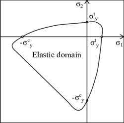
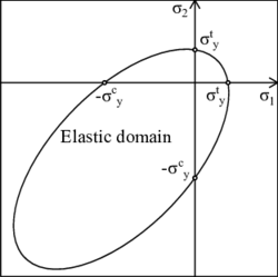
(a) Mazars.	(b) Modified von Mises.
Figure 1: Qualitative damage surfaces in the 2D principal stress space.

As one can see in Figure 1, the introduced forms of equivalent strain lead to non-symmetric damage surfaces in which the yield value in compression can be several times the value in tension. This is essential to account for the different strength in tension and compression of geo-materials such as concrete and rocks.

We summarize below the basic ingredients of the isotropic damage model:

• The stress-strain relation (1)
• The damage criterion, comprised by:
  • The loading function in (3)
  • The loading-unloading conditions in (5)
• The law governing the evolution of the damage variable (6)
• The expression defining the equivalent strain

3 Non-local damage model

Although isotropic damage models are quite simple, they are often used to model the failure of concrete and other quasi-brittle materials that show important strain localization. If the damage parameter depends only on the strain state at the point under consideration, the numerical simulations exhibit a pathological mesh dependence, and physically unrealistic results are obtained.

The introduction of a characteristic length into the constitutive model, and the formulation of a non-local strain-softening model, have been shown to prevent the spurious localization of strain-softening damage, to regularize the boundary value problem, and to ensure numerical convergence to physically meaningful solutions [4].

Integral-type non-local models abandon the classical assumption of locality and admit that stress at a certain point depends, not only on the state variables at that point, but also on the distribution of the state variables over the whole body, or over a finite neighbourhood of the point under consideration.

In a general manner, the non-local integral approach consists in replacing a certain variable by its non-local counterpart, obtained by weighted averaging over a spatial neighbourhood of each point under consideration.

Let ${\textstyle f({\boldsymbol {p}})}$ be some local field in a domain ${\textstyle V}$, the corresponding non-local field is defined as:

${\tilde {f}}({\boldsymbol {p}})=\int _{V}\alpha ({\boldsymbol {p}},{\boldsymbol {q}})f({\boldsymbol {q}})d{\boldsymbol {q}}$

(14)

where ${\textstyle \alpha ({\boldsymbol {p}},{\boldsymbol {q}})}$ is the chosen non-local weighting function.

In an infinite, isotropic and homogeneous medium, the weighting function depends only on the distance ${\textstyle D=\|{\boldsymbol {p}}-{\boldsymbol {q}}\|}$ between the source point ${\textstyle {\boldsymbol {q}}}$, and the receiver point ${\textstyle {\boldsymbol {p}}}$. Thereby, we usually write ${\textstyle \alpha ({\boldsymbol {p}},{\boldsymbol {q}})=\alpha _{0}(\|{\boldsymbol {p}}-{\boldsymbol {q}}\|)}$, where ${\textstyle \alpha _{0}(D)}$ is usually chosen as a non-negative function monotonically decreasing for ${\textstyle D\geq 0}$.

One possible choice for ${\textstyle \alpha _{0}(D)}$ is the Gauss distribution function:

$\alpha _{0}(D)=\exp \left[-\left({\frac {2D}{l_{c}}}\right)^{2}\right]$

(15)

where the characteristic length ${\textstyle l_{c}}$ is a material parameter reflecting the internal length of the non-local continuum.

If a bounded support is preferred, one can also truncate the previous function as follows:

$\alpha _{0}(D)=\left\{{\begin{array}{ll}\exp \left[-\left({\frac {2D}{l_{c}}}\right)^{2}\right]&{\hbox{ if }}|D|\leq R\\0&{\hbox{ if }}|D|>R\end{array}}\right.$

(16)

where the interaction radius ${\textstyle R}$ is a parameter usually related to the characteristic length ${\textstyle l_{c}}$. In the present work, we have considered ${\textstyle R=l_{c}}$.

In essence, the interaction radius ${\textstyle R}$ represents the smallest distance between points ${\textstyle {\boldsymbol {p}}}$ and ${\textstyle {\boldsymbol {q}}}$ at which the interaction weight ${\textstyle \alpha _{0}(\|{\boldsymbol {p}}-{\boldsymbol {q}}\|)}$ vanishes (for weighting functions with a bounded support) or becomes negligible (for weighting functions with an unbounded support). It represents a very important parameter because it controls the size of the softening region.

The interval, circle, or sphere of radius ${\textstyle R}$, centered at ${\textstyle {\boldsymbol {p}}}$, is called the domain of influence of point ${\textstyle {\boldsymbol {p}}}$ (Figure 2).

Figure 2: Averaging zone near the boundary of a solid.

In the application to softening materials, it is often required that the non-local operator do not alter a uniform field (consistency of order 0) which means that the weighting function must accomplish the normalizing condition:

${\begin{array}{cc}\displaystyle \int _{V}\alpha ({\boldsymbol {p}},{\boldsymbol {q}})d{\boldsymbol {q}}=1&\forall {\boldsymbol {p}}\in V\end{array}}$

(17)

In order to satisfy (17), the weighting function is rescaled as:

$\alpha ({\boldsymbol {p}},{\boldsymbol {q}})={\frac {\alpha _{0}(\|{\boldsymbol {p}}-{\boldsymbol {q}}\|)}{\displaystyle \int _{V}\alpha _{0}(\|{\boldsymbol {p}}-{\boldsymbol {x}}\|)d{\boldsymbol {x}}}}$

(18)

A suitable non-local damage formulation that restores well-posedness of the boundary value problem is obtained if damage is computed from the non-local equivalent strain [3].

In the loading function (3), the local equivalent strain ${\textstyle \varepsilon _{eq}}$ is replaced by its weighted spatial average:

${\tilde {\varepsilon }}_{eq}({\boldsymbol {p}})=\int _{V}\alpha ({\boldsymbol {p}},{\boldsymbol {q}})\varepsilon _{eq}({\boldsymbol {q}})d{\boldsymbol {q}}$

(19)

The internal state variable ${\textstyle r}$ is then the largest previously reached value of the non-local equivalent strain:

$r(t)=\max \left\{r_{0},\max _{\tau \leq t}{\tilde {\varepsilon }}_{eq}(\tau )\right\}$

(20)

It is important to note that the damage variable is evaluated from the non-local equivalent strain ${\textstyle {\tilde {\varepsilon }}_{eq}}$, whereas the strains ${\textstyle {\boldsymbol {\varepsilon }}}$ used in (1) to compute the stresses are considered as local. This way, during the elastic range, when the damage variable remains equal to zero, the stress-strain relation is fully local.

Numerical implementation of the non-local damage model based on averaging of the equivalent strain is relatively simple. The evaluation of the stresses remains explicit, and no internal iteration is needed. All that one needs is to implement the algorithm of weighted spatial averaging and, before damage is evaluated, replace the local equivalent strain by its non-local counterpart.

The values of the non-local equivalent strain must be traced at the individual Gauss integration points of the finite element mesh, because these are the points at which stresses are computed.

Thereby, the averaging integral in (19) is evaluated numerically. By considering the weighting function defined in (18) we can write:

${\tilde {\varepsilon }}_{eq,p}=\sum _{q}w_{q}\alpha _{pq}\varepsilon _{eq,q}$

(21)

where ${\textstyle w_{q}}$ is a coefficient containing the product of the determinant of the Jacobian and the integration weights of Gauss point ${\textstyle q}$, and ${\textstyle \alpha _{pq}}$ is the weight of non-local interaction between points ${\textstyle p}$ and ${\textstyle q}$, defined as:

$\alpha _{pq}={\frac {\alpha _{0}(\|{\boldsymbol {p}}-{\boldsymbol {q}}\|)}{\sum _{x}w_{x}\alpha _{0}(\|{\boldsymbol {p}}-{\boldsymbol {x}}\|)}}$

(22)

In the previous two equations, subscript ${\textstyle p}$ represents the receiver point under consideration, whereas indexes ${\textstyle q}$ and ${\textstyle x}$ correspond to source points. Since the chosen weighting function ${\textstyle \alpha _{0}}$ has bounded support (16), ${\textstyle \alpha _{pq}}$ vanishes if the distance between points ${\textstyle p}$ and ${\textstyle q}$ is larger than the interaction radius ${\textstyle R}$. Therefore, the sums in (21) and (22) do not need to be taken over all Gauss points, but only over those that are located inside the domain of influence of point ${\textstyle p}$.

In this regard, note that at the damage process zone one must always use an element size smaller than the interaction radius, in order to account for the non-local interaction. Otherwise the damage model would become local.

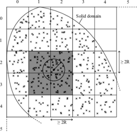
Each Gauss point must have a non-local interaction table that gives access to its neighbours. This table must be constructed at the beginning of the problem from a search of non-local neighbours. In this work, the search of neighbours is performed by means of a grid-based algorithm. A general rectangular grid is defined in the entire domain and all the integration points are positioned in the cells. This way, the neighbour search that must be performed for each Gauss point is restricted to a limited number of cells, i.e., the ones that fall inside the domain of influence of the considered point (Figure 3).

Figure 3: Grid-based non-local search.

The stress evaluation procedure, repeatedly called during the incremental-iterative strategy, makes use of the non-local interaction tables when the non-local equivalent strain is computed. To obtain ${\textstyle {\tilde {\varepsilon }}_{eq}}$ we first compute the local equivalent strains at all Gauss points, and then we calculate the non-local counterpart using (21).

4 Computation of the tangent stiffness matrix

If one aims to obtain an iterative solver with quadratic convergence when working with a non-local damage model, it is necessary to construct the tangent stiffness matrix in a consistent manner.

Let us start expressing the vector of internal forces as a numerical integration over the Gauss points. In order to make the explanation more understandable, from now on we will be using Voigt notation, i.e.

${\boldsymbol {f}}_{int}=\sum _{p}w_{p}{\boldsymbol {B}}_{p}^{T}{\boldsymbol {\sigma }}_{p}$

(23)

Using the stress-strain law (1) and the classic strain-displacement relation ${\textstyle {\boldsymbol {\varepsilon }}={\boldsymbol {B}}{\boldsymbol {a}}}$, we expand (23) as follows:

${\boldsymbol {f}}_{int}=\sum _{p}w_{p}(1-d_{p}){\boldsymbol {B}}_{p}^{T}{\boldsymbol {E}}{\boldsymbol {B}}_{p}{\boldsymbol {a}}$

(24)

The tangent stiffness matrix is obtained by differentiating the internal forces with respect to the vector of nodal displacements ${\textstyle {\boldsymbol {a}}}$. Since the damage variable depends on the nodal displacements through the equivalent strain, we will compute first the derivative of the damage variable with respect to the displacement vector ${\textstyle {\boldsymbol {a}}}$. Taking into account that ${\textstyle d=g(r)}$ (6), ${\textstyle r}$ depends on ${\textstyle {\tilde {\varepsilon }}_{eq}}$ (20), and ${\textstyle {\tilde {\varepsilon }}_{eq}}$ depends on ${\textstyle {\boldsymbol {a}}}$ through the interpolated strains, we use the chain rule to write the derivative of the damage variable for an integration point ${\textstyle p}$ as follows:

${\frac {\partial d_{p}}{\partial {\boldsymbol {a}}}}={\frac {dg}{dr_{p}}}{\frac {dr_{p}}{d{\tilde {\varepsilon }}_{eq,p}}}{\frac {\partial {\tilde {\varepsilon }}_{eq,p}}{\partial {\boldsymbol {a}}}}{=g'}_{p}t_{p}{\frac {\partial {\tilde {\varepsilon }}_{eq,p}}{\partial {\boldsymbol {a}}}}$

(25)

where ${\textstyle {g'}_{p}}$ is the derivative of the damage evolution law with respect to the internal state variable ${\textstyle r}$, and ${\textstyle t_{p}}$ is the loading-unloading factor that is 0 in an elastic loading or in an unloading regime, and 1 in a loading regime with growing damage. Thus,

$t_{p}=\left\{{\begin{array}{ll}0&{\hbox{ if }}{\tilde {\varepsilon }}_{eq,p}<r_{p}\\1&{\hbox{ if }}{\tilde {\varepsilon }}_{eq,p}=r_{p}{\hbox{ and }}{\dot {\tilde {\varepsilon }}}_{eq,p}\geq 0\end{array}}\right.$

(26)

Using expression (21), we can differentiate the non-local equivalent strain of a Gauss point ${\textstyle p}$ with respect to the nodal displacements as

${\frac {\partial {\tilde {\varepsilon }}_{eq,p}}{\partial {\boldsymbol {a}}}}=\sum _{q}w_{q}\alpha _{pq}{\frac {\partial \varepsilon _{eq,q}}{\partial {\boldsymbol {a}}}}=\sum _{q}w_{q}\alpha _{pq}{\frac {\partial \varepsilon _{eq,q}}{\partial {\boldsymbol {\varepsilon }}_{q}}}{\frac {\partial {\boldsymbol {\varepsilon }}_{q}}{\partial {\boldsymbol {a}}}}=\sum _{q}w_{q}\alpha _{pq}{\frac {\partial \varepsilon _{eq,q}}{\partial {\boldsymbol {\varepsilon }}_{q}}}{\boldsymbol {B}}_{q}$

(27)

The derivative of the equivalent strain with respect to the strain vector ${\textstyle \partial \varepsilon _{eq,q}/\partial {\boldsymbol {\varepsilon }}_{q}}$ is a row matrix that will depend on the chosen form of equivalent strain.

Let us now rewrite the expression of the internal forces in (24) as follows:

${\boldsymbol {f}}_{int}=\sum _{p}w_{p}{\boldsymbol {B}}_{p}^{T}{\boldsymbol {E}}{\boldsymbol {B}}_{p}{\boldsymbol {a}}-\sum _{p}w_{p}{\boldsymbol {B}}_{p}^{T}{\boldsymbol {E}}{\boldsymbol {B}}_{p}{\boldsymbol {a}}d_{p}$

(28)

At this point, we can already differentiate (28) and substitute (25) to get a first expression for the tangent stiffness matrix, as

${\boldsymbol {K}}_{tan}={\frac {\partial {\boldsymbol {f}}_{int}}{\partial {\boldsymbol {a}}}}$ $=\sum _{p}w_{p}{\boldsymbol {B}}_{p}^{T}(1-d_{p}){\boldsymbol {E}}{\boldsymbol {B}}_{p}-\sum _{p}w_{p}{\boldsymbol {B}}_{p}^{T}{\boldsymbol {E}}{\boldsymbol {B}}_{p}{\boldsymbol {a}}{g'}_{p}t_{p}{\frac {\partial {\tilde {\varepsilon }}_{eq,p}}{\partial {\boldsymbol {a}}}}$

(29)

Note that the first term in the right hand side (r.h.s.) of (29) is the secant stiffness matrix, that coincides with the tangent matrix in an elastic loading or in an unloading regime (${\textstyle t_{p}=0}$). The second term in the r.h.s. is the non-local part of the tangent stiffness matrix. Substituting (27) into (29) yields:

${\boldsymbol {K}}_{tan}={\boldsymbol {K}}_{sec}-\sum _{p}w_{p}{\boldsymbol {B}}_{p}^{T}{\boldsymbol {E}}{\boldsymbol {\varepsilon }}{_{p}g'}_{p}t_{p}\sum _{q}w_{q}\alpha _{pq}{\frac {\partial \varepsilon _{eq,q}}{\partial {\boldsymbol {\varepsilon }}_{q}}}{\boldsymbol {B}}_{q}$ $={\boldsymbol {K}}_{sec}-\sum _{p,q}w_{p}{\boldsymbol {B}}_{p}^{T}{\boldsymbol {\bar {\sigma }}}{_{p}g'}pw_{q}pw_{q}\alpha _{pq}{\frac {\partial \varepsilon _{eq,q}}{\partial {\boldsymbol {\varepsilon }}_{q}}}{\boldsymbol {B}}_{q}$

(30)

Defining for convenience the column matrix ${\textstyle {\boldsymbol {\beta }}_{p}^{c}={\boldsymbol {B}}_{p}^{T}{\boldsymbol {\bar {\sigma }}}_{p}}$, the row matrix ${\textstyle {\boldsymbol {\beta }}_{q}^{r}=\displaystyle {\frac {\partial \varepsilon _{eq,q}}{\partial {\boldsymbol {\varepsilon }}_{q}}}{\boldsymbol {B}}_{q}}$, and the coefficient ${\textstyle w_{pq}=w_{p}w_{q}\alpha _{pq}}$, Eq. (30) can be rewritten like:

${\boldsymbol {K}}_{tan}={\boldsymbol {K}}_{sec}-\sum _{p,q}{g'}_{p}t_{p}w_{pq}{\boldsymbol {\beta }}_{p}^{c}{\boldsymbol {\beta }}_{q}^{r}$

(31)

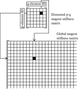
The double index of the sum, caused by the non-local interaction, implies that the term on the right part of Eq. (31) cannot be assembled from element contributions only. Essentially, each pair of Gauss points ${\textstyle p}$ and ${\textstyle q}$ contributes to the global stiffness matrix with a block of the same size as that of the classical element stiffness matrix. The difference is that the assembling routine differs from the usual one because in this case one needs to take into account the elements of both points ${\textstyle p}$ and ${\textstyle q}$ (Figure 4). Consequently, the global stiffness matrix is always non-symmetric and its bandwidth increases due to the non-local interaction.

Figure 4: Non-local assembly process.

In order to avoid the additional non-zero entries that the non-local interaction introduces into the global stiffness matrix, one could neglect the non-local terms by using ${\textstyle w_{pq}=\delta _{pq}w_{q}}$, where ${\textstyle \delta _{pq}}$ is the Kronecker delta. This way, Eq. (31) reduces to

${\boldsymbol {K}}_{tan}^{local}={\boldsymbol {K}}_{sec}-\sum _{p}{g'}_{p}t_{p}w_{p}{\boldsymbol {\beta }}_{p}^{c}{\boldsymbol {\beta }}_{p}^{r}$

(32)

where the sum is performed over one index only. Note that the resulting local tangent matrix ${\textstyle {\boldsymbol {K}}_{tan}^{local}}$ is no longer consistent, and quadratic convergence is lost.

Probably the most important issue caused by non-locality is the evolutionary character of the profile of the stiffness matrix. For the simulation of quasi-brittle materials like concrete, the consistent stiffness matrix remains local through the elastic branch, and so the initial distribution of non-zero entries is the same as in the local case. However, when the damage threshold is exceeded and the damage zone starts propagating, new non-zero entries appear due to the non-local interaction between Gauss points belonging to different elements, and the profile of the stiffness matrix must be dynamically adapted. The number of additional non-zero entries will depend on each particular case, but if a finer mesh is used in the expected softening zones, this number can be relatively high.

The non-local averaging certainly increases the computational cost with respect to the corresponding local model. However, the non-local model completely removes the pathological sensitivity to the mesh size and partially alleviates the mesh-induced directional bias. Consequently, this extra computational effort is indeed worthwhile.

5 Mesh-adaptive technique

In this work we have used the error estimation and adaptive mesh refinement strategy presented by Oñate and co-workers [5, 6, 27-29].

The general algorithm of non-linear adaptive FEM analysis implemented in this work is described as follows. After reaching the equilibrium state and updating the solution, an error estimation is performed in order to evaluate the error distribution over the mesh. Then, a remeshing criterion uses the information about error distribution and determines the required mesh density. From this analysis, we obtain a new spatial discretization using a mesh generator interface.

In a truly adaptive approach, after generating a new discretization, the data structures corresponding to the newly generated mesh are created, and the transfer of displacements and internal variables from the old mesh to the new one is performed. After the mapping, the internal variables are used together with the strain computed from the mapped displacements to update the internal state of each integration point on the new mesh (to achieve local consistency). Once the transfer has finished, the old discretization is deleted and the mapped configuration is brought into global equilibrium through iteration. Afterwards, the solution continues with the next incremental-iterative step.

Another possibility is to restart the analysis from the initial state after the new discretization is generated. This approach does not require the transfer of the current state from the old discretization to the new one, but from the computational point of view is less efficient than the truly adaptive approach, especially if the remeshing is done frequently.

We present below the main stages of the implemented adaptive procedure:

5.1 Error estimation

The error estimator is based on the stress evaluation. We define the error as the difference between an exact value of the effective stresses ${\textstyle {\bar {\boldsymbol {\sigma }}}_{e}}$ and an approximate one ${\textstyle {\bar {\boldsymbol {\sigma }}}_{a}}$:

${\boldsymbol {\epsilon }}_{\bar {\sigma }}={\bar {\boldsymbol {\sigma }}}_{e}-{\bar {\boldsymbol {\sigma }}}_{a}$

(33)

Note that we compute the error with the effective stresses ${\textstyle {\bar {\boldsymbol {\sigma }}}}$ and not with the total stresses ${\textstyle {\boldsymbol {\sigma }}}$ because the latter tend to zero as damage grows.

A reasonably good value of the exact stresses is obtained from their extrapolation from the Gauss points to the nodes and a posterior smoothing [27]. The approximate value of stresses is simply the default evaluated stresses of the FEM solution. Therefore, the estimated error can be defined as the difference between the smoothed effective stresses ${\textstyle {\bar {\boldsymbol {\sigma }}}_{s}}$, and the calculated effective stresses ${\textstyle {\bar {\boldsymbol {\sigma }}}}$:

${\boldsymbol {\epsilon }}_{\bar {\sigma }}\approx {\bar {\boldsymbol {\sigma }}}_{s}-{\bar {\boldsymbol {\sigma }}}$

(34)

We will work with integral measures of the error. The energy norm of the error over an element is defined as:

$\|{\boldsymbol {\epsilon }}_{\bar {\sigma }}\|^{(e)}=\left[\int _{\Omega ^{(e)}}{\boldsymbol {\epsilon }}_{\bar {\sigma }}^{T}{\boldsymbol {E}}^{-1}{\boldsymbol {\epsilon }}_{\bar {\sigma }}d\Omega \right]^{1/2}$ $=\left[\int _{\Omega ^{(e)}}[{\bar {\boldsymbol {\sigma }}}_{s}-{\bar {\boldsymbol {\sigma }}}]^{T}{\boldsymbol {E}}^{-1}[{\bar {\boldsymbol {\sigma }}}_{s}-{\bar {\boldsymbol {\sigma }}}]d\Omega \right]^{1/2}$

(35)

The square of the global error can be obtained from the sum of the squares of all the elemental errors:

$\|{\boldsymbol {\epsilon }}_{\bar {\sigma }}\|^{2}=\sum _{e}(\|{\boldsymbol {\epsilon }}_{\bar {\sigma }}\|^{(e)})^{2}$

(36)

The smaller is the distance between the nodes of the mesh, the smaller will be the difference between the smoothed and non-smoothed stresses. Thereby, the presented energy norm tends to zero as the size of the element diminishes, i.e., ${\textstyle \|{\boldsymbol {\epsilon }}_{\bar {\sigma }}\|={\mathcal {O}}(h^{m})}$ where ${\textstyle h}$ is the element size and ${\textstyle m}$ is the order of the polynomial defining the shape functions.

5.2 Remeshing

Determining whether a mesh must be refined or not requires to previously define some quality conditions based on the estimated error.

First, the energy norm of the global error should be smaller than a certain percentage of the deformation energy:

$\|{\boldsymbol {\epsilon }}_{\bar {\sigma }}\|\leq \eta \,U$

(37)

where ${\textstyle \eta }$ is the permissible percentage of global error, prescribed a priori, and the deformation energy is obtained from:

$U^{2}=\sum _{e}(U^{(e)})^{2}$

(38)

with

$U^{(e)}=\left[\int _{\Omega ^{(e)}}{\bar {\boldsymbol {\sigma }}}_{s}^{T}{\boldsymbol {E}}^{-1}{\bar {\boldsymbol {\sigma }}}_{s}d\Omega \right]^{1/2}$

(39)

To determine whether condition (37) is fulfilled, it is convenient to work with a global error parameter defined as:

$\xi _{g}={\frac {\|{\boldsymbol {\epsilon }}_{\bar {\sigma }}\|}{\eta \,U}}$

(40)

Thereby, when ${\textstyle \xi _{g}=1}$ the global error condition is perfectly fulfilled. For ${\textstyle \xi _{g}>1}$ the mesh should be refined, and for ${\textstyle \xi _{g}<1}$ the average mesh size could be larger.

Taking into account that ${\textstyle \|{\boldsymbol {\epsilon }}_{\bar {\sigma }}\|={\mathcal {O}}(h^{m})}$, the new element size ${\textstyle {\hat {h}}^{(e)}}$ can be obtained with:

${\hat {h}}^{(e)}={\frac {h^{(e)}}{(\xi _{g})^{\frac {1}{m}}}}$

(41)

If one aims at obtaining a selective refinement method, apart from (37), another condition concerning the error of each element must be simultaneously imposed. In this paper, we have chosen a remeshing criterion based on a global error equidistribution [28].

This criterion distributes the global error uniformly among all the elements of the mesh, and so the elemental error must accomplish the following condition:

$\|{\boldsymbol {\epsilon }}_{\bar {\sigma }}\|^{(e)}\leq {\frac {\|{\boldsymbol {\epsilon }}_{\bar {\sigma }}\|}{\sqrt {n}}}$

(42)

where ${\textstyle n}$ is the number of elements of the mesh.

Like for the global error, we can work with a local error parameter:

$\xi _{l}^{(e)}={\frac {{\sqrt {n}}\,\|{\boldsymbol {\epsilon }}_{\bar {\sigma }}\|^{(e)}}{\|{\boldsymbol {\epsilon }}_{\bar {\sigma }}\|}}$

(43)

with the same meaning that in the global case: ${\textstyle \xi _{l}^{(e)}=1}$ indicates an optimal element size, whereas ${\textstyle \xi _{l}^{(e)}>1}$ and ${\textstyle \xi _{l}^{(e)}<1}$ imply that the element is too large and too small, respectively.

This local parameter allows us to define the new element size that accomplishes (42):

${\hat {h}}^{(e)}={\frac {h^{(e)}}{(\xi _{l}^{(e)})^{\frac {2}{2m+d}}}}$

(44)

where ${\textstyle d}$ is the space dimension of the problem.

In the end, the remeshing criterion results from the combination of the global error condition (37) and the local one (42). In consequence, the final refinement parameter of the element can be defined as:

$\xi ^{(e)}=\xi _{g}\,\xi _{l}^{(e)}={\frac {{\sqrt {n}}\,\|{\boldsymbol {\epsilon }}_{\bar {\sigma }}\|^{(e)}}{\eta \,U}}$

(45)

And the new element size is obtained with:

${\hat {h}}^{(e)}={\frac {h^{(e)}}{\gamma ^{(e)}}}$

(46)

where

$\gamma ^{(e)}=(\xi _{g})^{\frac {1}{m}}\,(\xi _{l}^{(e)})^{\frac {2}{2m+d}}$

(47)

5.3 Mesh generator interface

The mesh generator interface is the pre-processing and post-processing GiD software used to run the simulations [1]. Therefore, not only GiD meshes the geometry at the beginning of the numerical solution, but it is also GiD which allows to obtain the new spatial discretization every time we need to adapt the mesh.

Thereby, after the error estimator and the remeshing criterion are applied, a "background mesh" file is generated with the information of the new element sizes. Then, GiD allows us to load this background mesh file along with the original mesh file so as to generate a new mesh according to the refinement parameter of each old element.

5.4 Mapping of variables

Before one can continue with the solution of a problem, there is a last stage that must be performed in a truly adaptive approach: the mapping of primary unknowns and internal variables.

In essence, if one aims at continuing the analysis from the current state, instead of restarting it from scratch after every mesh refinement, it is necessary to apply some transfer algorithms for the displacements and internal history variables (in the present case, the state variable ${\textstyle r}$ governing the damage evolution).

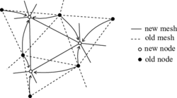
Mapping of the primary unknowns (nodal displacements) is achieved by using the shape function projections. To do so, we must first place each new node inside an old element, by means of a grid-based search, and then we interpolate the displacements of the old nodes to the new ones (Figure 5a).

Mapping of the internal state variables is done through a weighted spatial averaging, similar to the one used for the computation of the non-local equivalent strain. The difference is that, in this case, the source points are the integration points of the old mesh, and the receiver points are the integration points of the new mesh (Figure 5b). Once again, another grid-based search is performed in order to determine the Gauss points of the old mesh that fall inside the interaction radius ${\textstyle R}$ of each new Gauss point.

(a) Nodal displacements mapping.

(b) Internal state variables mapping.

Figure 5: Mapping of variables.

6 Examples

In this section we will present two examples of application of the non-local damage model and the mesh adaptive technique proposed. The examples are the three-point bending test and the four-point shear test. For each case we will first assess the robustness of the non-local damage model when working with different spatial discretizations, and then we will solve the problem again applying the mesh-adaptive technique, in order to point out the strengths and limitations of the code in its current state.

Regarding the solving strategy, we will be following the equilibrium path of the problem for a series of steps through a global arc-length method in an incremental-iterative process. Self weight will not be considered.

6.1 Three-point bending test

This test is performed with a notched beam subjected to three-point bending (TPB). The beam has a square cross section of 40 ${\textstyle \times }$ 320 mm, a span of 1280 mm. The notch is 3 mm thick and extends over one tenth of the beam depth (Figure 6).

Figure 6: TPB test. Problem statement. Distances in mm

Plane stress conditions have been assumed. The geometry was meshed by 4-noded quadrilaterals with 2 ${\textstyle \times }$ 2 integration points.

Non-local damage model solution

As it has been stated before, the non-local damage model was defined with the Mazars model, regarding the equivalent strain (12) and the damage evolution law (7). The material parameters were obtained from [17] and are summarized in Table 1.

Table. 1 TPB test. Material parameters for Mazars non-local damage model.

Parameter	Value
Young modulus (${\textstyle E}$)	38500 MPa
Poisson's ratio (${\textstyle \nu }$)	0.24
Damage threshold (${\textstyle r_{0}}$)	${\textstyle 3\cdot {10}^{-5}}$
Parameter ${\textstyle A}$ in compression (${\textstyle A_{c}}$)	1.25
Parameter ${\textstyle B}$ in compression (${\textstyle B_{c}}$)	1000
Parameter ${\textstyle A}$ in tension (${\textstyle A_{t}}$)	0.95
Parameter ${\textstyle B}$ in tension (${\textstyle B_{t}}$)	9000
Characteristic length (${\textstyle l_{c}}$)	40 mm

In order to assess the robustness of the non-local damage model, we have also solved the problem with a local damage model based on the damage evolution law of [24] and a modified definition of the equivalent strain presented by Simo and Ju in [33]. The parameters for this model are shown in Table 2.

Table. 2 TPB test. Material parameters for Simo-Ju local damage model.

Parameter	Value
Young modulus (${\textstyle E}$)	38500 MPa
Poisson's ratio (${\textstyle \nu }$)	0.24
Compressive strength (${\textstyle \sigma _{y}^{c}}$)	45 MPa
Tensile strength (${\textstyle \sigma _{y}^{t}}$)	3.8 MPa
Fracture energy (${\textstyle G_{f}}$)	100 ${\textstyle J/m^{2}}$
Limit fracture length (${\textstyle l_{lim}}$)	5 mm

The problem was solved for different spatial discretizations. In this case we used three unstructured meshes of 4-noded quadrilaterals with a minimum size of 15 mm, 7 mm, and 3 mm, respectively (Figure 7).

(a) Mesh 1: 2024 4-noded elements.

(b) Mesh 2: 2679 4-noded elements.

(c) Mesh 3: 6543 4-noded elements.

Figure 7: TPB test. Spatial discretizations.

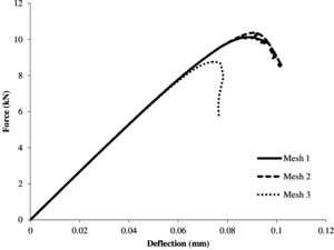
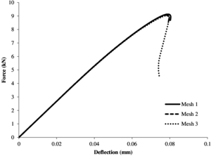
Figure 8 shows the relation between the applied load and the vertical deflection of the beam for each mesh. As one can see from the discontinued equilibrium curves, we had serious difficulties in tracing the response of a full test. The reason behind the convergence problems could be the use of a too global arc-length method. Indeed, to account for the localized nature of quasi-brittle failure, a more specific control parameter, like the Crack Mouth Opening Displacement (CMOD), could help improving the convergence near snap-back zones.

That aside, if we look at the curves in Figure 8a we can see that, although there is no relevant difference between the response obtained with meshes 1 and 2, the peak load actually decreases with the finest mesh 3, and so the total dissipated energy. On the other hand, the response diagram in Figure 8b shows practically the same peak load for the three meshes.

(a) Local damage model.

(b) Non-local damage model.

Figure 8: TPB test. Force-vertical deflection diagrams.

Figure 9 shows clearly the different behaviour of the local and non-local approaches. While in the local model the thickness of the damage pattern is of the order of the element size, in the non-local case the damage pattern is controlled by the interaction radius ${\textstyle R}$ and so the response remains virtually unaltered regardless of the mesh.

(a) Local model. Initial stage.	(b) Non-local model. Initial stage.
(c) Local model. Middle stage.	(d) Non-local model. Middle stage.
(e) Local model. Advanced stage.	(f) Non-local model. Advanced stage.
Figure 9: TPB test. Evolution of damage propagation.

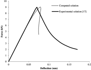
Furthermore, in order to check whether the implemented model can properly reproduce the behaviour of the real test, we have compared the results obtained in the non-local model with experiments performed in [17].

Figure 10 shows the force-vertical deflection diagram of the experimental solution and the computed solution with mesh 3.

Figure 10: TPB test. Non-local model validation.

As we can see, the peak load is properly captured, but the post peak branch of the numerical solution falls faster than in the experimental solution, and even shows a certain amount of snap-back behaviour. Looking at the elastic branch of the responses, it seems that the stiffness degradation starts before in the computed solution and, in consequence, the peak is slightly displaced to the right. Therefore, we can say that the behaviour of the numerical model seems more brittle than that observed in the experiment. This difference could be due to the approach used in the laboratory test to control the post-peak behaviour.

Mesh-adaptive solution

The same problem was solved again, using the mesh-adaptive technique described along with the non-local damage model.

As mentioned in Section 5.2, we use a remeshing criterion based on the global error equidistribution. The objective of the example was to obtain efficient spatial discretizations for the changing damage states, limiting the global error to a 10% of the deformation energy ${\textstyle (\eta =10\%)}$. The initial mesh is an unstructured mesh of 4-noded quadrilaterals with an average size of 10 mm.

In this case three refinements have been performed. In order to understand the mesh-adaptive process, it is interesting to see the evolution of damage for the different meshes (Figure 11).

(a) Mesh 0: 4453 4-noded elements. $\xi _{g}=1.33$

(b) Mesh 1: 2977 4-noded elements. $\xi _{g}=0.67$

(c) Mesh 2: 1598 4-noded elements. $\xi _{g}=0.92$

(d) Mesh 3: 1627 4-noded elements. $\xi _{g}=0.93$

Figure 11: TPB test. Progression of damage in the adaptive mesh.

A quantitative measure of the suitability of the mesh is given by the global refinement parameter ${\textstyle \xi _{g}}$. A value close to 1 means that the global error is similar to the goal percentage of error ${\textstyle \eta }$. The value of 1.33 in Figure 11a denotes that the mesh must be refined in those areas of the structure with higher stress variations, i.e., the zone near the notch, the point of application of the load, and the supports. On the other hand, since this procedure also optimizes the mesh enlarging the elements on those zones with smoother stresses, the number of elements can be reduced from 4453 to 2977.

In the subsequent meshes (Figures 11b, 11c and 11d) the global refinement parameters are smaller than 1, showing that the mesh-adaptive technique properly keeps the error below the prescribed threshold.

We can say that the main advantage of the adaptive mesh technique is that it automatically optimizes the mesh for the problem we are solving, so that the number of elements can be drastically reduced, and so the computational cost of the problem. However, this procedure still does not distinguish compressive stresses from tensile stresses when estimating the error. In materials like concrete, this can lead to excessively small elements in compressed zones, and so it could be convenient to give more weight to the tensile stresses.

6.2 Four-point shear test

The test will be performed with a single-edge notched beam subjected to four-point shear (FPS). The analysed beam has a square cross section of 100 ${\textstyle \times }$ 200 mm, a span of 840 mm, and the notch is 10 mm thick and 40 mm depth (Figure 12).

Figure 12: FPS test. Problem statement. Distances in mm

Plane stress conditions have been assumed. The geometry was meshed using standard linear 3-noded triangles with one integration point.

Non-local damage model solution

The non-local damage model is defined with the equivalent strain form of the modified von Mises model (13), and the simplified exponential damage evolution law (11). The material parameters for the non-local approach have been obtained from [32] and are summarized in Table 3.

Table. 3 FPS test. Material parameters for modified von Mises non-local damage model.

Parameter	Value
Young modulus (${\textstyle E}$)	28000 MPa
Poisson's ratio (${\textstyle \nu }$)	0.1
Damage threshold (${\textstyle r_{0}}$)	${\textstyle 1.5\cdot {10}^{-4}}$
Compressive to tensile strength ratio (${\textstyle \kappa }$)	10
Parameter ${\textstyle A}$ (${\textstyle A}$)	0.8
Parameter ${\textstyle B}$ (${\textstyle B}$)	9000
Characteristic length (${\textstyle l_{c}}$)	10 mm

Like in the first example, we have compared the non-local damage model with a local damage model (Table 4).

Table. 4 FPS test. Material parameters for Simo-Ju local damage model.

Parameter	Value
Young modulus (${\textstyle E}$)	28000 MPa
Poisson's ratio (${\textstyle \nu }$)	0.1
Compressive strength (${\textstyle \sigma _{y}^{c}}$)	35 MPa
Tensile strength (${\textstyle \sigma _{y}^{t}}$)	3.2 MPa
Fracture energy (${\textstyle G_{f}}$)	140 ${\textstyle J/m^{2}}$
Limit fracture length (${\textstyle l_{lim}}$)	5 mm

In this case, we used three unstructured meshes of 3-noded triangles with a minimum size of 8 mm, 5 mm, and 3 mm, respectively (Figure 13).

(a) Mesh 1: 2216 3-noded elements.

(b) Mesh 2: 3502 3-noded elements.

(c) Mesh 3: 7183 3-noded elements.

Figure 13: FPS test. Spatial discretizations.

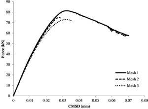
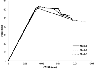
In Figure 14 we represent the relation between the applied load and the Crack Mouth Sliding Displacement (CMSD) for each mesh. The curves in Figure 14a show that in this case the peak and the dissipated energy also decrease as the mesh is refined. However, this reduction is not so clear as in the previous example. On the other hand, Figure 14b shows virtually the same peak load for the three meshes. Also, although we can notice some oscillations in the post-peak regions of meshes 1 and 2, we can say that the residual force at the right part of the graph seems to be pretty similar for all cases.

(a) Local damage model.

(b) Non-local damage model.

Figure 14: FPS test. Force-Crack Mouth Sliding Displacement diagrams.

Figure 15 shows the damage progression for both models stressing the more localized nature of the local damage model. Regarding the non-local model, if we compare this example with the three-point bending test, we can clearly see that the damage progression zone here is restricted to a narrower region than before. The reason is that now the characteristic length defining the interaction radius is quite smaller than before.

(a) Local model. Initial stage.	(b) Non-local model. Initial stage.
(c) Local model. Middle stage.	(d) Non-local model. Middle stage.
(e) Local model. Advanced stage.	(f) Non-local model. Advanced stage.
Figure 15: FPS test. Evolution of damage propagation.

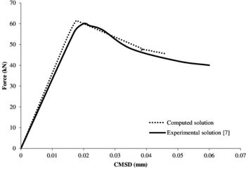
Figure 16 shows the relation between the applied load and the Crack Mouth Sliding Displacement of a reference experimental solution [7] and the computed solution with the finest mesh.

Figure 16: FPS test. Non-local model validation.

We can see that the obtained response is very similar to the experimental solution. What should be noticed, though, is that the failure obtained in the computed solution is slightly more brittle as compared to the experimental one. This is possibly consequence of an imprecise tracing of the equilibrium path, caused by the global arc-length strategy used.

Mesh-adaptive solution

This example is performed with the same permissible percentage of global error as in the previous one ${\textstyle (\eta =10\%)}$, but the initial mesh is an unstructured mesh of triangles with an average size of 7 mm.

In this case the number of refinements is four. The evolution of damage for the different spatial discretizations is represented in Figure 17.

(a) Mesh 0: 7784 3-noded elements. $\xi _{g}=1.84$

(b) Mesh 1: 6800 3-noded elements. $\xi _{g}=1.05$

(c) Mesh 2: 6590 3-noded elements. $\xi _{g}=2.20$

(d) Mesh 3: 10626 3-noded elements. $\xi _{g}=0.44$

(e) Mesh 4: 2542 3-noded elements. $\xi _{g}=0.94$

Figure 17: FPS test. Progression of damage in the adaptive mesh.

Figure 17a shows no damage before the first refinement. It can be deduced then that the subsequent spatial discretization is mainly caused by the high compressive stresses at the loading points and at the supports.

However, from Figures 17c, 17d and 17e it is clear that the adaptive procedure properly captures the damage process zone and adapts the mesh accordingly.

Another aspect to consider here is directly related to the abrupt failure of the computed solution seen in Figure 16. Indeed, when damage grows abruptly the global refinement parameter ${\textstyle \xi _{g}}$ increases up to a value of 2.20 (Figure 17c). Consequently, the adaptive technique refines excessively all the affected zone, leading to a considerably large number of elements and a much smaller global refinement parameter (Figure 17d). Nonetheless, once damage progress stabilises, the adaptive procedure readjusts the spatial discretization and the resulting mesh is actually efficient (Figure 17e).

Finally, we can notice that the damage pattern in Figure 17e is a bit wider than the one shown in Figure 15f. The reason could be that some extra damage diffusion is introduced due to the errors appearing during the transfer of internal variables between meshes. Therefore, in the near future it would be important to assess the effect of these errors in the traced equilibrium path, and improve the transfer algorithms if necessary.

7 Conclusions

The implemented non-local damage model has shown a robust behaviour for changing spatial discretizations, avoiding pathological mesh sensitivity and mesh-induced directional bias. It has also proved to properly capture the experimental peak load of the response diagrams in the two examples analysed: the three-point bending test and the four-point shear test. However, the numerical solution has shown a more brittle post-peak branch as compared to the experimental results. An important aspect to note about this integral-type non-local approach is that the averaging performed to account for the non-local interaction, considerably increases the computational cost of the solution, as compared to the classical local approach, and also modifies the traditional assembly process of the global tangent stiffness matrix.

That aside, it must be stated that the global arc-length strategy used in the simulations has shown an irregular success when tracing the non-linear solution, and so it is probably not the best approach for the kind of problems we have been solving. Indeed, the implementation of an advanced arc-length method with a specific control parameter (CMOD or CMSD) that accounts for the localized nature of quasi-brittle materials could help improving the accuracy of the converged solution.

The implemented mesh-adaptive technique allows one to capture the process damage zone and adjust the spatial discretization accordingly. This procedure generates large elements in zones with smooth stress distribution, and small elements in zones with strong variations of stresses. Hence, efficient mesh distributions can be obtained. Nevertheless, the mesh adaptive technique is still a recent implementation and there are some features that will be improved in subsequent work. For instance, the procedure does not distinguish compressive stresses from tensile stresses when estimating the error, which can result in excessively fine meshes at compressed zones that are not actually transcendent for the damage progression of materials like concrete. Furthermore, errors in the transfer operations of internal variables introduce some extra damage diffusion that should be analysed in order to assess its influence in the traced equilibrium path.

Acknowledgements

The authors are thankful to Mr. Miquel Portabella for his collaboration in the implementation of the mesh-adaptive technique.

This research was partially funded by the Advanced Grant project SAFECON of the European Research Council and project NUMEXAS of the FP7 of the European Commission.

References

[1] GiD the personal pre and post processor. http://www.gidhome.com/, April 2015.

[2] Z. P. Bazant, T. B. Belytschko, and T.-P. Chang. Continuum theory for strain-softening. Journal of Engineering Mechanics, 110(12):1666- 1692, 1984.

[3] Z. P. Bazant and M. Jirásek. Nonlocal integral formulations of plasticity and damage: survey of progress. Journal of Engineering Mechanics, 128(11):1119-1149, 2002.

[4] Z. P. Bazant and G. Pijaudier-Cabot. Nonlocal continuum damage, localization instability and convergence. Journal of applied mechanics, 55(2):287-293, 1988

[5] G. Bugeda and E. Oñate. Adaptive mesh refinement techniques for aerodynamic problems. In Proceedings of the International Conference on Métodos Numéricos en Ingeniería y Ciencias Aplicadas. Universidad de Concepción, Chile. 16-20 November 1992, pages 513-522. Published by CIMNE, Barcelona, 1992.

[6] G. Bugeda and E. Oñate. A methodology for adaptive mesh refinement in optimum shape design problems. Computing Systems in Engineering, 5(1):91-102, 1994.

[7] A. Carpinteri, S. Valente, G. Ferrara, and G. Melchiorrl. Is mode ii fracture energy a real material property? Computers & structures, 48(3):397-413, 1993.

[8] M. Cervera and M. Chiumenti. Mesh objective tensile cracking via a local continuum damage model and a crack tracking technique. Computer Methods in Applied Mechanics and Engineering, 196(1):304-320, 2006.

[9] M. Cervera, M. Chiumenti, and C. A. de Saracibar. Shear band localization via local j 2 continuum damage mechanics. Computer Methods in Applied Mechanics and Engineering, 193(9):849-880, 2004.

[10] J. De Vree, W. Brekelmans, and M. Van Gils. Comparison of nonlocal approaches in continuum damage mechanics. Computers & Structures, 55(4):581-588, 1995.

[11] A. C. Eringen. On nonlocal plasticity. International Journal of Engineering Science, 19(12):1461-1474, 1981.

[12] A. C. Eringen and D. Edelen. On nonlocal elasticity. International Journal of Engineering Science, 10(3):233-248, 1972

[13] M. Fafard and B. Massicotte. Geometrical interpretation of the arc-length method. Computers & structures, 46(4):603-615, 1993

[14] J. Hult. Creep in continua and structures. In Topics in applied continuum mechanics, 137-155, 1974.

[15] M. Jirásek and S. Rolshoven. Comparison of integral-type nonlocal plasticity models for strain-softening materials. International Journal of Engineering Science, 41(13):1553-1602, 2003.

[16] L. Kachanov. On the time of fracture under conditions of creep. Izv. AN SSSR, Otd. Tekh. Nauk, (8):26-35, 1958.

[17] C. Le Bellego and É. normale supérieure de Cachan. Couplages chimie-mécanique dans les structures en béton attaquées par l'eau: Etude expérimentale et analyse numérique. LMT-ENS Cachan, 2001.

[18] J. Lemaitre and J. Chaboche. Mécanique des matériaux solides, 1985. Dunod, Paris.

[19] B. Loret and J. H. Prevost. Dynamic strain localization in elasto-(visco-) plastic solids, part 1. general formulation and one-dimensional examples. Computer Methods in Applied Mechanics and Engineering, 83(3):247-273, 1990

[20] J. Mazars. Application de la mécanique de l'endommagement au comportement non linéaire et à la rupture du béton de structure. PhD thesis, 1984.

[21] J. Mazars. A description of micro-and macroscale damage of concrete structures. Engineering Fracture Mechanics, 25(5):729-737, 1986.

[22] J. Mazars and G. Pijaudier-Cabot. From damage to fracture mechanics and conversely: a combined approach. International Journal of Solids and Structures, 33(20):3327-3342, 1996.

[23] H. Mühlhaus. Shearband analysis in antigranulocytes material by cosserat-theory. Ingenieur Archiv, 56(5):389-399, 1986.

[24] J. Oliver, M. Cervera, S. Oller, and J. Lubliner. Isotropic damage models and smeared crack analysis of concrete.In Second International Conference on Computer Aided Analysis And Design of Concrete Structures, volume 2, 945-958, 1990

[25] J. Oliver, M. Cervera, S. Oller, and J. Lubliner. A simple damage model for concrete, including long term effects. In Second International Conference on Computer Aided Analysis And Design of Concrete Structures, volume 2, 945-958, 1990

[26] S. Oller, E. Oñate, J. Oliver, and J. Lubliner. Finite element nonlinear analysis of concrete structures using a ‘’plastic-damage model’’. Engineering Fracture Mechanics, 35(1):219-231, 1990.

[27] E. Oñate. Structural Analysis with the Finite Element Method. Linear Statics: Volume 1: Basis and Solids, volume 1. Springer Science & Business Media, 2009.

[28] E. Oñate and G. Bugeda. A study of mesh optimality criteria in adaptive finite element analysis. Engineering Computations, 10(4):307-321, 1993.

[29] E. Oñate and J. Castro. Adaptive mesh refinement techniques for structural problems. In The finite element method in the 1990's, 133-145. Springer, 1991.

[30] G. Pijaudier-Cabot and Z. P. Bazant. Nonlocal damage theory. Journal of Engineering Mechanics, 113(10):1512-1533, 1987

[31] Y. Rabotnov. Damage from creep. Zhurn. Prikl. Mekh. Tekhn. Phys, 2:113-123, 1963

[32] A. Rodríguez Ferran, I. Arbós, A. Huerta, et al. Adaptive analysis based on error estimation for nonlocal damage models. 2001.

[33] J. Simo and J. Ju. Strain-and stress-based continuum damage models-i. formulation. International journal of solids and structures, 23(7):821-840, 1987.

[34] H. Zbib and E. Aifantis. A gradient-dependent ow theory of plasticity: application to metal and soil instabilities. Applied Mechanics Reviews, 42(11S):S295-S304, 1989.