ABSTRACT=
In this work a finite element method (FEM) is proposed to solve the problem of estimating the added resistance of a ship in waves in the time domain and using unstructured meshes. Two different schemes are used to integrate the corresponding free surface kinematic and dynamic boundary conditions: the first one based on streamlines integration (SLI); and the second one based on the Streamline-Upwind Petrov-Galerking (SUPG) stabilization. The proposed numerical schemes have been validated in different test cases, including towing tank tests with monochromatic waves. The results obtained in this work show the suitability of the present method to estimate added resistance in waves in a computationally affordable manner.
Keywords: Added resistance in waves, FEM, unstructured mesh, potential flow.
1. Introduction
In order to get a good prediction of the total resistance of a ship in a seaway the added resistance in waves has to be taken into account. And although the added resistance in waves is a second order component, it may reach up to 40% of the total average resistance for some specific wave frequencies where wave radiation increases.
Despite of the importance of the added resistance in waves and its impact on the long term performance of a ship, there are not many works in the literature coping with this problem using computational methods. Some formulation have been derived by different authors as an extension of the mean drift force induced by waves in the presence of a water current (Maruo 1957; Journée 1992). These approaches basically modify damping and added mass coefficients, as well as the mean drift forces, to account for the current effect. However, convective terms in the free surface boundary conditions are neglected, limiting this approach to low Froude numbers. A more sophisticated approach is to solve the three dimensional potential flow problem in the frequency domain using the boundary element method (BEM), and obtain the added resistance using Maruo’s approach thereafter (Maruo 1960; Maruo 1963; Liu at al. 2011). However, Maruo’s approach is still limited to low Froude numbers, since it does not account for the free surface convective terms either. Few works can be found trying to solve the added resistance in waves in the time domain considering the convective terms in the free surface boundary condition and using potential flow (Joncquez 2009; Seo et al. 2013; Afshar 2014; Park et al. 2016). The latter approaches are based on the BEM, consider linearized convective terms, and are constrained to structured meshes.
Non-linear viscous CFD solvers have also been applied to analyze details of the added resistance in waves (Sadat-Hosseini et al. 2013; el Moctar et al. 2015;Tezdogan et al. 2015; Kim et al. 2017a; kim et al. 2017b; Kim et al. 2017c; Ozdemir and Barlas 2017; Hizir et al. 2018). Recently Sigmund and el Moctar (2018) carried out state of the art numerical and experimental investigations on four types of ships using the finite volume method. The effect on added resistance of the ship's speed, wave steepness, skin friction and diffraction-radiation was analyzed in detail. Among other findings, it was found that: calm water and added resistance must be computed on the same numerical grid; radiation forces are more influenced by the ship's speed than by the diffraction forces; in short waves and at model scale frictional resistance accounts for some 20% of the total added resistance, while this percentage is not as high for full scale; and, finally, that the assumption of a quadratic dependence of added resistance on wave amplitude holds for moderate and long waves, while it does not in short waves because wave diffraction is dominant. However, since the use of CFD tools is computationally expensive, its application is limited to research analysis. On the other hand, potential flow solver are more suitable to evaluate systematically a large number of navigation conditions.
The main motivation of this work is the development of a new time-domain computational model capable of solving the wave making and added resistance problem efficiently. This can be achieved by offering am accurate approach not subject to the use of structured meshes.
The proposed method is based on potential flow and applies the free surface boundary conditions on the mean water level for computational efficiency. The main novelties of the model are the use of the Finite Element Method (FEM) on unstructured meshes (Servan-Camas and Garcia-Espinosa 2013, Garcia-Espinosa et al. 2015; Servan-Camas 2016; Oñate et al. 2018) in the context of potential flow. The proposed numerical scheme is derived using a non-linear (NL) formulation for the convective terms, although the Neumann-Kelvin (NK) and double-body (DB) flow linearizations have been analyzed as well.
The first scheme proposed for integrating the free surface boundary conditions is based on computing the convective term as a derivative along the streamlines. To this end a third order finite difference (FD) scheme using three points upwind and one point downwind has been tailored. The second scheme proposed is based on the FEM with Streamline-Upwind Petrov-Galerkin (SUPG) stabilization (Brooks and Hughes 1982).
2. Mathematical models for wave resistance problems
2.1 Problem statement
We consider the first-order diffraction-radiation problem of a body moving on the horizontal plane. Potential flow is assumed and the problem is formulated in terms of the velocity potential and free surface elevation. The following assumptions are made on the order of magnitude of the velocity components and free surface elevation:
|
(1) | |
|
where the velocity potential, ξ is is the free surface elevation, is the forward speed of the moving body and is the uniform water current vector. The velocity potential and free surface elevation are split into incident and diffraction-radiation components:
|
(2) | |
|
(3) |
where and are the diffraction-radiation velocity potential and free surface elevation, and and are the incident wave potential and free surface elevation (modeled as a set of Airy waves).
2.2 Governing equations in a moving frame of reference
The governing equations are solved in a frame of reference fixed to the moving body. Let the two dimensional movement of the local frame be defined by the horizontal velocity (see Figure 1). This frame of reference is assumed to match the global frame at time zero. For an observer sitting on the ship the flow field around is given by the relative motion . Then the first-order diffraction-radiation equations in the local frame of reference are (see Servan-Camas 2016):
|
(4) | |
|
(5) | |
|
(6) | |
|
(7) | |
|
(8) |
where , is the body surface below , is the velocity of a point P on , and is the water depth The pressure induced by diffracted and radiated waves is
|
(9) |

|
2.3 Flow linearization
The previous governing equations have been obtained under the assumption . Then the free surface boundary conditions remain non-linear and can be written as follows
|
(10) | |
|
(11) |
where represents the convective velocity and must be updated every iteration to account for the variations of and . Retaining this assumption allows for simulating flows where is not steady. However, linearization of the convective velocity is a common practice when is steady and under assumptions of low speed or slender bodies. Two commonly used linearizations are:
The NK linearization: assumes . Then the convective velocity becomes the apparent velocity .
The DB linearization: assumes with and . The flow field is obtained from the double-body approximation (see Servan-Camas 2016).
2.4 Second-order pressure correction over body
A second-order correction on the pressure calculation is proposed in order to better estimate hydrodynamic loads. The idea is to retain second-order terms depending on the first-order solution. Although this will not provide a full second-order solution, it will retain the terms contributing to mean drift loads ( ), and added resistance in waves ( ). The second-order pressure correction is:
|
|
(12) |
where and are pressures induced by the incident and diffracted-radiated waves respectively, is the first-order displacement of a point P over the body surface, and is the pressure correction term. The first term of the right hand side account for the pressure variation due to first order movements, and the second term accounts for second-order terms depending on first-order terms.
2.5 Second-order pressure correction on waterline
The movements of a ship and the free surface elevation modify the wetted surface. In order to take into account this change, a linear pressure is assumed from the waterline to the free surface (see Figure 2):
|
(13) | |
|
|
(14) |
where and are evaluated at z=0, is the first-order pressure at z=0, and represents the vertical pressure distribution over the water line (see Servan-Camas 2016).

3. Numerical schemes
3.1 Problem statement
Let be the finite element (FE) space of interpolating functions, defined in the usual manner. From this space we can construct the subspace that incorporates the Dirichlet conditions for the velocity potential . The space of test functions, denoted by , is constructed as , but with functions vanishing on the boundary where the Dirichlet conditions are imposed. Then the discrete variational finite element problem associated with the Eqs. (27)-(31) can be written as follows (Belibassakis et al. 2013): Find , by solving
|
(15) |
where , , are the potential normal gradients corresponding to the Neumann boundary conditions on bodies, radiation boundary and free surface, respectively. At this point it is useful to introduce the associated matrix form (Zienkiewicz et al. 2005a)
|
(16) |
where is the standard FE Laplacian matrix, and is a vector accounting for the right hand side of the dynamic condition of the free surface, and and are the vectors resulting from integrating the other boundary condition terms.
Two different schemes have been developed to integrate the free surface boundary conditions (Eq. (10) and Eq. (11)): one based on FD streamline integration (FD-SLI), and the other based on FEM with SUPG stabilization scheme (FEM-SUPG). Both schemes have been tailored to account for the non-linear convective terms and to be used on unstructured meshes.
3.2 FD-SLI
The first-order free surface boundary conditions can be written in a general form as follows:
|
(17) | |
|
(18) |
where and represent remaining terms depending on the linearization used. The numerical schemes adopted for solving the kinematic-dynamic free surface boundary conditions are based on Adams-Bashforth-Moulton schemes, using an explicit scheme for the kinematic condition, and an implicit one for the dynamic condition. Then is imposed as a Dirichlet boundary condition. The schemes read as follows:
|
(19) | |
|
(20) |
where is the convective velocity and the convective terms are evaluated by differentiating along streamlines as:
|
|
(21) | |
|
|
where denotes the derivative along the streamline. This streamline derivative is estimated using a two points upstream and one point downstream FD operator. Figure 3 shows the tracing of the streamline at node 0. The left (-1) and forward left (-2) points are upstream points, while the right (1) point corresponds to the downstream point. Then the streamline differential operator reads as:
|
|
(22) | |
|
|
where , , are interpolated between , , and respectively. In matrix form, the resulting scheme can be written as:
|
(23) | |
|
(24) |
where and are the streamline convective and identity matrices respectively. The stencils are tailored using Taylor series expansion to get a third-order FD scheme along the streamline.
The associated matrix form to the FE formulation for the governing equations is:
|
(25) |
where is the standard Laplacian matrix modified to account for the left hand side of Eq.(23), is a vector containing the right hand side of Eq. (23), and and are the vectors resulting from integrating the other boundary condition terms.

3.3 FEM-SUPG
Alternatively a FEM-SUPG (Hughes and Mallet 1986) has been also developed for integrating the free surface boundary conditions. The dynamic and kinematic boundary conditions can be seen as convective-transport equations of the form:
|
|
(26) |
The standard FE problem associated to the above equation is
|
|
(27) |
where is the corresponding shape function associated to the mesh node and and represent the values of and at node , respectively. The above equation is discretized in time as follows:
|
|
(28) |
where . It is well known that the numerical solution of the previous equation may show spurious oscillations (Zienkiewicz et al. 2005b; Donea and Huerta 2003). Hence the SUPG formulation is used to introduce the necessary stabilization. The resulting scheme is
|
(29) |
In matrix form:
|
(30) |
Where
|
(31) |
The FEM-SUPG dynamic and kinematic boundary conditions become
|
(32) | ||
|
|
(33) | ||
In this work an explicit ( ) and implicit ( ) schemes are used for the kinematic and dynamic conditions respectively. The matrix form associated to the FE formulation of the governing equations is:
|
(34) |
where is the standard Laplacian matrix modified to account for the left hand side of Eq. (32), is a vector accounting for the right hand side of Eq. (32), and and are the vectors resulting of integrating the other boundary condition terms.
4. Hydrodynamic loads for wave resistance problems
4.1 First-order loads
Hydrodynamic forces and moments are obtained from direct pressure integration over the body surface (Bai and Teng 2013). The body gravity center ( ) will be used as a reference for body movements and moments acting on it. The resulting expressions for forces ( ) and moments ( ) can be found in (Servan-Camas 2016).
4.2 Second-order correction
Second-order correction loads are obtained by calculating the components of the second-order loads depending on the first-order solution as described in section 2.5 (Figure 2). Integrating the corresponding second-order pressure correction:
|
|
(35) | |
|
|
(36) |
The mean value of the longitudinal component of has a special meaning in the presence of waves: when it becomes the mean drift force due to the waves; and when it becomes the added resistance in waves. Additionaly second-order correction of dynamic and hydrostatic loads resulting from the first-order rotation (see Servan-Camas 2016) are also taken into account in this work.
5. Verification and validation
5.1 Wave making resistance of an elliptic pressure distribution
5.1.1 Problem description
Newman and Poole (1962) derived an analytical solution for the wave resistance of a pressure distribution moving with constant forward speed along the free surface of a canal with constant width and depth. This solution was obtained based on a first-order approximation with uniform flow (NK). In particular, an analytical expression for the elliptic pressure distribution was obtained. The main particulars of the elliptic pressure distribution used to validate the present model are given in Table 1:
| Length (L) | 1 m |
| Beam (B) | 0.5 m |
| Water depth (H) | 5 m |
| Channel width (W) | 10 m |
| Free surface pressure ( ) | 1 Pa |
The wave resistance is obtained by integrating the pressure distribution over the free surface as follows:
|
|
(37) |
It is assumed that the pressure distribution moves in the x direction. Then, in order to obtain the wave resistance, it is mandatory to be able to estimate the free surface deformation within the pressure patch.
5.1.2 Convergence analysis
Different unstructured meshes have been used for the numerical calculations. It has been found that refinement at the edge of the pressure distribution is mandatory due to the discontinuity in the pressure and its large influence in the free surface deformation, especially at low Froude numbers where wave lengths are smaller. Table 2 provides the particulars for each mesh and Figure 4 shows a detail of the finest one.
| Pressure patch edge (m) | Pressure patch (m) | Free surface outside (m) | Volume (m) | |
| Mesh 1 | 0.002 | 0.02 | 0.02 | 0.05 |
| Mesh 2 | 0.003 | 0.03 | 0.03 | 0.075 |
| Mesh 3 | 0.004 | 0.04 | 0.04 | 0.1 |
| Mesh 4 | 0.006 | 0.06 | 0.06 | 0.15 |
| Mesh 5 | 0.008 | 0.08 | 0.08 | 0.20 |
Wave resistance was calculated for all the meshes at Froude number Fr=0.2, using the FD-SLI and FEM-SUPG schemes presented in sections 3.2 and 3.3 respectively. Table 3 provides the values of the relative errors. Figure 5 shows the free surface elevation computed for Fr=0.2 with the FEM-SUPG and the finer mesh.
| Analytical =0.1840 | Mesh 5 | Mesh 4 | Mesh 3 | Mesh 2 | Mesh 1 | |
| Streamline | 1.550 | 1.640 | 1.730 | 1.780 | 1.820 | |
| Error | 15.77 % | 10.88 % | 5.99 % | 3.27 % | 1.10 % | |
| FEM-SUPG | 1.643 | 1.710 | 1.775 | 1.795 | 1.820 | |
| Error | 10.74 % | 7.08 % | 3.54 % | 2.46 % | 1.10 % | |


5.1.3 Verification
The wave making resistance has been calculated for several Froude numbers for the finest mesh using the FD-SLI and FEM-SUPG. Table 4 compares analytical and numerical results. It can be observed that the numerical results are able to reproduce the analytical ones with small errors.
| Fr | |||
| FD-SLI | FEM-SUPG | Analytical
(Newman and Poole 1962) | |
| 0.2 | 1.82 | 1.82 | 1.84 |
| 0.3 | 2.18 | 2.16 | 2.18 |
| 0.4 | 1.67 | 1.65 | 1.64 |
| 0.5 | 2.73 | 2.66 | 2.66 |
5.2 Wave making resistance of a Wigley hull
5.2.1 Problem description
The wave making resistance of a Wigley hull is analyzed. Different simulations have been performed considering the NL, NK, and DB free surface conditions. The FD-SLI and FEM-SUPG schemes have been used for integrating the free surface boundary conditions. Wave resistance coefficients with and without second-order correction have been obtained.
The standard Wigley hull with beam to length ratio B/L=0.1 and amidships section coefficient Cm=0.6667 was used. An unstructured mesh was generated with an element size around the ship of 0.01 m. The mesh generated consists of 84351 nodes and 476083 tetrahedral elements (see Figure 6). Only half domain was required due to the symmetry of the problem.

5.2.2 Second-order correction and flow linearizations
Figure 7 compares the dimensionless first-order wave making resistance coefficients and the dimensionless second-order-corrected wave making resistance coefficients . They have been obtained using the NL, NK and DB assumptions for the case of a fixed Wigley hull model in still water. The wave making resistance forces and have been calculated as the longitudinal forces obtained by pressure integration (section 4). It is observed that the increase of resistance due to the second-order correction term is noticeable.
The NK linearization leads to smaller values of wave resistance when compared to the NL and DB approaches, while the NL and DB predict similar results up to Fr=0.3.

Figure 7: Wave resistance for Wigley hull using NL, DB, and NK approximations. Dimensionless first-order wave making resistance ( ), and dimensionless second-order-corrected wave making resistance ( ).
5.2.3 Validation
Figure 8 compares the second-order-corrected numerical results obtained in this work with NL flow approximation against several experimental results: ITTC (1984) (collection of experimental data), Shearer and Cross (1965), University of Iowa, University of Tokyo (UT), and the Ship Research Institute of Japan (SRI). The results from Iowa, UT and SRI can be found in Ju (1983). Experimental data shows large dispersion and this might be mainly due to the uncertainty of model testing and the assumption of a constant form factor with speed.
Taking into account the large dispersion of the experimental data a fairly good agreement between the numerical and the experimental results has been obtained. This agreement is better for the higher Froude numbers. Lower Froude numbers require a much finer discretization in order to reproduce the shorter wave pattern. Figure 9 compares the wave profiles at the water line obtained numerically against experimental results. A good agreement is also found in this case.


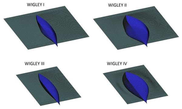
5.3 Added resistance in waves of four modified Wigley hulls
5.3.1 Problem description
In this section computed added resistance is compared to that obtained by Journée (1992). Journée carried out an extensive model test campaign measuring the added resistance in waves of four modified Wigley hulls.. The main particulars of the models are given in Table 5.
| Wigley I | Wigley II | Wigley III | Wigley IV | |
| Amidships section coefficient Cm | 0.9090 | 0.9090 | 0.6667 | 0.6667 |
| Length to breadth ratio, L/B | 10 | 5 | 10 | 5 |
| Length L (m) | 1 | 1 | 1 | 1 |
| Breadth B (m) | 0.1 | 0.2 | 0.1 | 0.2 |
| Draught d (m) | 0.0625 | 0.0625 | 0.0625 | 0.0625 |
| Displacement (m3) | 0.003504 | 0.007008 | 0.002889 | 0.005778 |
| KG (m) | 0.05667 | 0.0625 | 0.05667 | 0.0625 |
| Radius of inertia for pitch, kyy (m) | 0.25 | 0.25 | 0.25 | 0.25 |
| Pitch damping (N/(m/s)) |
5.3.2 Validation
The added resistance has been estimated by subtracting the second-order-corrected longitudinal force in still water to the average value of the second-order-corrected longitudinal force obtained in the presence of a monochromatic wave. Then the dimensionless wave resistance is calculated as:
|
|
(38) |
where A is the wave amplitude.
Simulations have been carried out with the streamlines and FEM-SUPG scheme using the NL flow approximations. Pitch damping was introduced to model the viscous dissipation effects, and prevent the excessive pitch movement around resonance obtained otherwise (see Table 5). The amount of damping introduced was calibrated to best fit the RAOs response across all Froude numbers tested.
Journée (1992) reported that in some case studies (for instance Wigley II at Fr=0.3 and Fr=0.4) it was not possible to stabilize the experiments, and therefore no results were obtained in those cases. This gives an idea on the complexity of carrying out this type of experiments, and the uncertainty that might be involved (Park et al. 2015). Moreover the added resistance in waves is a second-order force and usually quite small when compared to first-order forces, which makes very complicate to measure and separate both quantities. In fact, quite large models are needed to be able to measure second order forces, which is not the case of the referred experiments where the model length was 3 m. Since experimental data might have significant uncertainties, such results must be analyzed qualitatively rather than quantitatively.
Figure 10 shows a snapshot of the wave pattern generated by the Wigley III hull at Fr=0.2 advancing against a monochromatic wave with a wave length equal to the length of the hull. Figure 11 provides the time evolution of the resistance in still water and in wave for the same case. The added resistance can be obtained from the difference between the still water resistance and the mean value of the resistance in wave. Figure 12 shows the hull geometries and mesh sizes used.
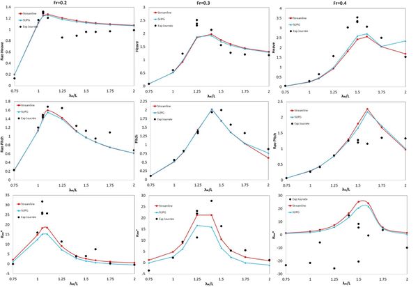
Figure 13-16 show the heave and pitch RAOs, as well as the dimensionless added resistance , versus the dimensionless wavelength for the four modified Wigley hull models.
Overall the results obtained with the FD-SLI and the FEM-SUPG schemes are quite similar to each other. Only in a few cases slight deviations are observed. Regarding the experimental results general trends are well captured, although in some cases some scattering is observed. Numerical results for RAOS and added resistance in waves follow reasonably well the experimental data although the goodness of the fitting depends on each case. Resonance frequencies are recovered well although peak values of added resistance are often underestimated.

 
|


6. Summary and conclusion
A FEM based model to compute the wave making resistance in still water and added resistance in waves has been proposed. The proposed method solves the governing equations in the time-domain, using unstructured meshes, and is not constrained to linearized free surface boundary conditions. The mathematical model is based on potential and Stokes’ perturbation method, which makes it computationally attractive compared to CFD solvers. Two different numerical schemes have been proposed to solve the free surface boundary conditions: the first one is based on a third order FD-SLI scheme using three upwind plus one downwind points; and the second one is based on the FEM-SUPG stabilization.
The proposed schemes have been verified comparing against analytical solutions available for a moving pressure patch, and validated against experimental results by comparing wave making resistance and wave profiles. The verification and validation analyses have proved that fairly good results are obtained by the FD-SLI and FEM-SUPG schemes.
Regarding the use of linearized convective terms, the following conclusions are made: the NK linearization might be valid for low Froude numbers (lower than 0.15), but it is not advisable for higher velocities, even for slender bodies like the Wigley hull; wave making resistance predictions using the DB linearization are quite close to the NL approach.
The numerical results of added resistance in waves have been validated against experimental data available for four modified Wigley hulls at different Froude numbers and for a number of monochromatic waves. Added resistance highly depend on the wave induced heave and pitch movements, requiring a good calibration of the viscous damping is mandatory. The added resistance in waves is a second-order force and quite small when compared to first-order forces, which makes it very complicate to measure experimentally. In fact quite large models are needed to be able to measure second order forces, which is not the case of the refereed experiments where the model length was 3 m. Hence experimental data has significant uncertainties and its results must be analyzed qualitatively rather than quantitatively. Taking this into account, it can be concluded that the present methodology has been capable of estimating fairly well heave and pitch RAOs, and the added resistance trends.
Acknowledgements
This research work was partially supported by the X-SHEAKS project (ENE2014-59194-C2-1-R) of the Ministerio de Economía y Competitividad (Spain).
REFERENCES
Afshar, M. (2014). Towards predicting the added resistance of slow ships in waves. Ph.D. Thesis, Technical University of Denmark.
Bai, W., & Teng, B. (2013). Simulations of second-order wave interaction with fixed and floating structures in time domain. Ocean Engineering, 74, 168-177.
Belibassakis, K., Gerostathis, T., Kostas, K., Politis, C., Kaklis, P., Ginnis, A., & Feurer, C. (2013). A BEM isogeometric method for the ship wave-resistance problem. Ocean Engineering, 60, 53-67.
Brooks, A., & Hughes, T. (1982). Streamline upwind/Petrov-Galerkin formulations for convection dominated floaws with particular emphasis on the incompressible Navier-Stokes equations. Computer Methods in Applied Mechanics and Engineering, 32, 199-259.
Donea, J., & Huerta, A. (2003). Finite element methods for flow problems. John Wiley & Sons, Ltd. doi:10.1002/0470013826.
el Moctar, O., Sigmund, S., & Schelling, T. (2015). Numerical and experimentla analysis of added resistance of ships in waves. Proceedings of the ASME 34th International Conference on Ocean, Offshore and Artic Engineering OMAE 2015. St. John´s, NL, Canada.
Hizir, O., Kim, M., Turan, O., Day, A., & Incecik, A. (2018). Numerical studies on non-linearity of added resistance and ship motions of KVLCC2 in short and long waves. International Journal of Naval Architecture and Ocean Engineering, 1-11.
ITTC84. (1984). Report of Resistance Comitee. Göteborg: Proceeding of the 17th International Towing Tank Conference.
Joncquez, S. (2009). Second-order forces and moments acting on ships in waves. Ph.D. Thesis, Technical University of Denmark.
Journée, J. (1992). Experiments and calculations on 4 Wigley hull forms in head waves. Delft University of Technology. Report 0909.
Ju, S. (1983). Study of total viscous drag for the Wigley parabolic ship form. IIHR Report no. 261.
Kim, M., Hizir, O., Turan, O., & Incecik, A. (2017a). Numerical studies on added resistance and motions of KVLCC2 in head seas for various ship speeds. Ocean Engineering, 140, 466-476.
Kim, M., Hizir, O., Turan, O., Day, S., & Incecik, A. (2017b). Estimation of added resistance and ship speed loss in a seaway. Ocean Engineering, 141, 465-476.
Kim, Y.-C., Kim, K.-S., Kim, J., Kim, Y., Park, I.-R., & Jang, Y.-H. (2017c). Analysis of added resistance and seakeeping responses in head sea conditions for low-speed full ships using URANS approach. International Journal of Naval Architecture and Ocean Engineering, 9, 614-654.
Liu, S., Papanikolaou, A., & Zaraphonitis, G. (2011). Prediction of added resistance in waves. Ocean Engineering, 38, 614-650.
Maruo, H. (1957). The excess resistance in rough seas. International Shipbuilding progress, 4(35).
Maruo, H. (1960). The drift of a body floating on waves. Journal of Ship Research., 4(3), 1-10.
Maruo, H. (1963). Resistance in waves. 60th Anniversary Series. 8, pp. 67-102. The Society of Naval Architects of Japan.
Newman, J., & Poole, F. (1962). The wave resistance of a moving pressure distribution in a canal. David Taylor Model Basin, Report 1619.
Oñate, E., García-Espinosa, J., Idelsohn, S., & Serván-Camas, B. (2018). Ship hydrodynamics. In Encyclopedia of Computational Mechanics Second Edition. John Wiley & Sons, Ltd. doi:10.1002/9781119176817.
Ozdemir, Y., & Barlas, B. (2017). Numerical study of ship motions and added resistance in regular incident waves of KVLCC2 model. International Journal of Naval Architecture and Ocean Engineering, 9, 149e159.
Park, D.-M., Kim, Y., Seo, M.-G., & Lee, J. (2016). Study on added resistance of a tanker in head waves at different drafts. Ocean Engineering, 111, 569-581.
Park, D.-M., Lee, J., & Kim, Y. (2015). Uncertainty analysis for added resistance experiment o fKVLCC2 ship. Ocean Engineering, 95, 143-156.
Sadat-Hosseini, H., Wu, P.-C., Carrica, P., Kim, H., Toda, Y., & Stern, F. (2013). CFD verification and validation of added resistance and motions of KVLCC2 with fixed and free surge in short and long head waves. Ocean Engineering, 59, 240-273.
Seo, M.-G., Park, D.-M., Yang, K.-K., & Kim, Y. (2013). Comparative study of ship added resistance in waves. Ocean Engineering, 73, 1-15.
Servan-Camas, B. (2016). A time-domian finite element method for seakeeping and wave resistance problems. Doctoral Thesis, ETSI Navales, Universidad Politecnica de Madrid. http://oa.upm.es/39794/1/BORJA_SERVAN_CAMAS.pdf
Servan-Camas, B., & Garcia-Espinosa, J. (2013). Accelerated 3D multi-body seakeeping simulation using unstructured finite elements. Journal of Computational Physics, 252, 382-403.
Sigmund, S., & el Moctar, O. (2018). Numerical and experimental investigation of added resistance of
different ship types in short and long waves. Ocean Engineering, 147, 51-67.
Shearer, J., & Cross, J. (1965). The experimental determination of the components of ship resistance for a mathematical model. Transactions of teh Royal Institution of Naval Architecs, 107, 459-473.
Tezdogan, T., Demirel, Y., Kellett, P., Khorasanchi, M., & Incecik, A. (2015). Full-scale unsteady RANS CFD simulations of ship behaviour and performance in head seas due to slow steaming. Ocean Engineering, 97, 186-206.
Zienkiewicz, O., Taylor, R., & Nithiarasu, P. (2005a). The finite element method for fluid dynamics. Elsevier butterworth-Heinemann.
Zienkiewicz, O., Taylor, R., & Zhu, J. (2005b). The finite element metho: its basis and fundamentals (sixth edition). Elsevier butterworth-Heinemann.
Document information

Published on 01/01/2018
DOI: 10.1080/17445302.2018.1483624
Licence: CC BY-NC-SA license
